In this section we discuss how MTEX aligns coordinate systems on the screen and how to change it. In MTEX it is possible to mix different alignment. At the same time MTEX tries to be as consistent as possible, e.g. by aligning EBSD maps and pole figures with respect to the same reference directions.
Different alignments are typically used when
- displaying directions in crystal vs. specimen reference frame
- displaying orthogonal 2d EBSD sections
In MTEX each plottable variable has a property how2plot
v1 = vector3d(1,1,1);
v2 = vector3d(-1,1,1);
v1.how2plot
ans = plottingConvention (y↑→x)
outOfScreen: (0,0,1)
north : (0,1,0)
east : (1,0,0)The property how2plot is a handle class of type plottingConvention and tells MTEX how to align the corresponding coordinate system on screen.
plot(v1,'label','v_1','figSize','small')
annotate([xvector,yvector,zvector],'labeled','backgroundcolor','w')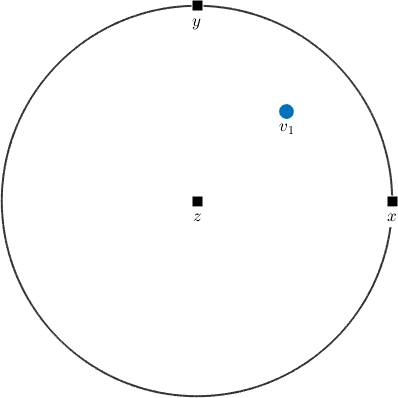
We can change it by setting north, east or outOfScreen to other directions.
v1.how2plot.outOfScreen = yvector
plot(v1,'label','v_1','figSize','small')
annotate([xvector,yvector,zvector],'labeled','backgroundcolor','w')v1 = vector3d (z↓→x)
x y z
1 1 1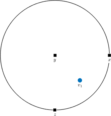
Note that plottingConvention is a handle class, i.e. changing v1.how2plot changes also v2.how2plot
v2.how2plot
plot(v2,'label','v_2','figSize','small')
annotate([xvector,yvector,zvector],'labeled','backgroundcolor','w')ans = plottingConvention (z↓→x)
outOfScreen: (0,1,0)
north : (0,0,-1)
east : (1,0,0)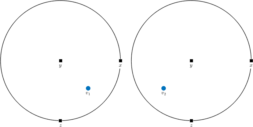
In order to have different plotting axes alignments within one MTEX session we have to define a new plottingConvention by
% instantiate a new plotting convention and sets it up
pC2 = plottingConvention; pC2.north = yvector
% assign this plottingConvention to v2
v2.how2plot = pC2;
% plot v1 and v2 in separate plots
plot(v1,'upper','label','v_1')
annotate([xvector,yvector,zvector],'labeled','backgroundcolor','w')
nextAxis
plot(v2,'upper','label','v_2')
annotate([xvector,yvector,zvector],'labeled','backgroundcolor','w')pC2 = plottingConvention (y↑→x)
outOfScreen: (0,0,1)
north : (0,1,0)
east : (1,0,0)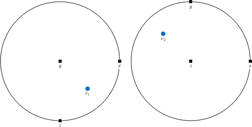
When initiating a new vector3d MTEX uses plottingConvention.default as default plotting convention. This default plotting convention can be changed by
plotx2north
plotzOutOfPlane
plot([xvector,yvector,zvector],'upper','labeled','backgroundcolor','w')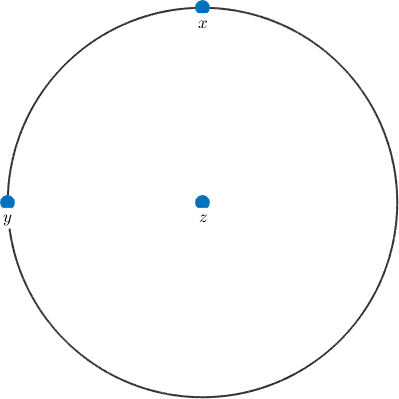
When importing data those might be associated with a plotting convention that is different to the default one
mtexdata dubna
pf.how2plot
plot(pf{1:4})pf = PoleFigure (y↑→x)
crystal symmetry : Quartz (321, X||a*, Y||b, Z||c*)
h = (022̅1), r = 72 x 19 points
h = (101̅0), r = 72 x 19 points
h = (101̅1)(011̅1), r = 72 x 19 points
h = (101̅2), r = 72 x 19 points
h = (112̅0), r = 72 x 19 points
h = (112̅1), r = 72 x 19 points
h = (112̅2), r = 72 x 19 points
ans = plottingConvention (y↑→x)

  outOfScreen: (0,0,1)
  north      : (0,1,0)
  east       : (1,0,0)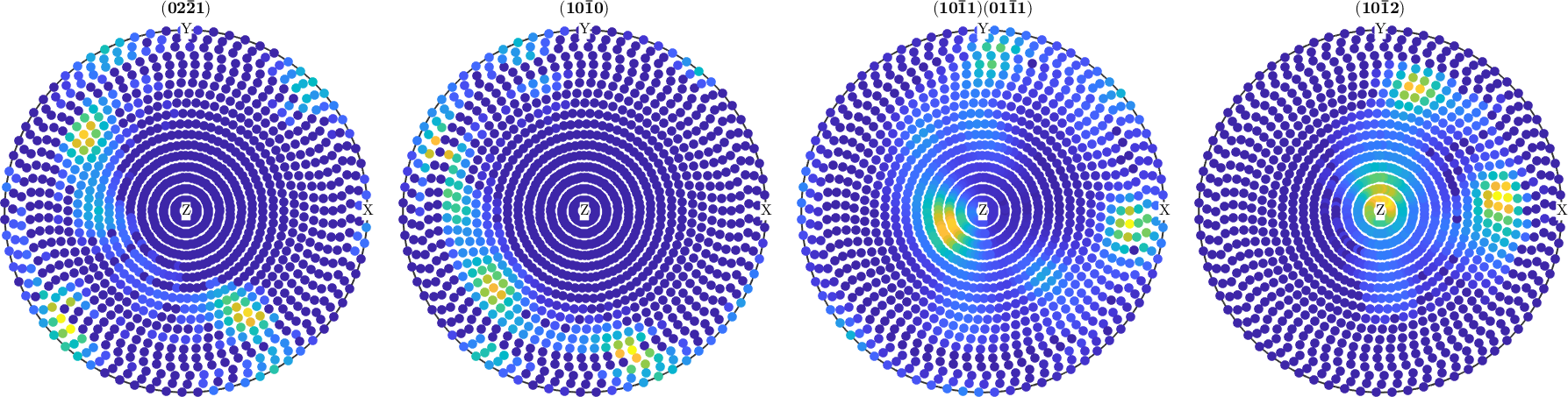
Note that all quantities derived from those data will inherit the stored plotting convention
odf = calcODF(pf,'silent');

plotPDF(odf,pf.allH{1:4})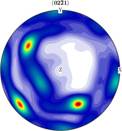
We may also set the default plotting convention to the plotting convention of the imported data by
pf.how2plot.makeDefault
plottingConvention.default
ans = plottingConvention (y↑→x)
outOfScreen: (0,0,1)
north : (0,1,0)
east : (1,0,0)