A fibre in orientation space is the equivalent of straight lines in Euclidean space, it is the shortest path between any two orientations. In MTEX it is defined by the command fibre.
% consider cubic symmetry
cs = crystalSymmetry('432');

% two random orientations
oriA = orientation.rand(cs)
oriB = orientation.rand(cs)

% this is important to have the pair of orientations with the smallest distance
oriB = oriB.project2FundamentalRegion(oriA)

% define the connecting fibre
f = fibre(oriA,oriB)

plot(oriA,'axisAngle','filled','MarkerSize',20)
hold on
plot(oriB,'axisAngle','filled','MarkerSize',20)

hold on
plot(f,'lineWidth',3,'lineColor','red')
hold off
axis off
oriA = orientation (432 → y↑→x)
Bunge Euler angles in degree
phi1 Phi phi2
156.958 161.468 197.878
oriB = orientation (432 → y↑→x)
Bunge Euler angles in degree
phi1 Phi phi2
156.716 99.1642 118.921
oriB = orientation (432 → y↑→x)
Bunge Euler angles in degree
phi1 Phi phi2
262.796 149.782 288.448
f = fibre (432 → y↑→x)
h || r: (9̅7̅3̅) || (-2,7,4)
o1 → o2: (157°,161.5°,197.9°) → (262.8°,149.8°,288.4°)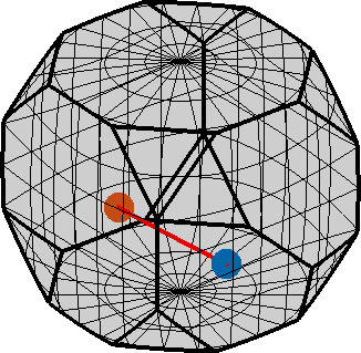
Due to the curved nature of the orientation space it is better to understand fibers not as straight lines but as big circles on a sphere. That is, if we extend them they will form a loop of length 2*pi. In MTEX this is done by the option 'full'.
f = fibre(oriA,oriB,'full')

hold on
plot(f,'lineWidth',3,'lineColor','red')
hold off
f = fibre (432 → y↑→x)
h || r: (9̅7̅3̅) || (-2,7,4)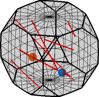
The strange multiple lines in the above pictures are all from the same circle that has been projected into the fundamental zone by crystal symmetry. If we dismiss crystal symmetry and visualize the complete rotation space we observe that f is indeed a circle.
plot(oriA,'axisAngle','filled','MarkerSize',20,'complete')
hold on
plot(oriB,'axisAngle','filled','MarkerSize',20)

plot(f,'axisAngle','lineWidth',3,'lineColor','red')
axis off
hold off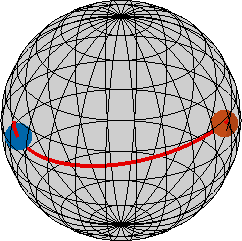
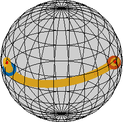
Another way of characterizing fibers is that they are the set of all orientations that that align a specific crystal direction h with a specific specimen direction r. Those directions can be read from the fiber f by
f.r
f.h
ans = vector3d (y↑→x)
x y z
-0.243 0.839 0.487
ans = Miller (432)
h k l
-0.77 -0.5887 -0.2461Note that f.h and f.r are exactly the misorientation axes between the orientations oriA and oriB
% the axis in specimen symmetry
r = axis(oriB,oriA)

% the axis in crystal symmetry
h = inv(oriA) * axis(oriB,oriA)
r = vector3d (y↑→x)
x y z
-0.243 0.839 0.487
h = Miller (432)
h k l
-0.77 -0.5887 -0.2461We may use h and r directly to define a fibre within MTEX by
f = fibre(h,r)f = fibre (432 → y↑→x)
h || r: (9̅7̅3̅) || (-2,7,4)A discretization of such a fibre can be found using the command orientation
ori = orientation(f)

% plot the rotations along the fibre
hold on
plot(ori)
hold off
ori = orientation (432 → y↑→x)
size: 2000 x 1