Importing Vectors

A direction file is only a table of numbers until its coordinate columns are identified. vector3d.load turns those columns into a vector3d array.

This page assumes that polar angle and azimuth are familiar. See Defining Three-Dimensional Vectors for their definitions and for the distinction between vectors and directions.

plottingConvention.default('y↑→x');

Reading a File

The example file contains one direction per row. Its first numeric column is the polar angle, and its second is the azimuth, both in degrees.

fname = fullfile(mtexDataPath,'vector3d','vectors.txt');

v = vector3d.load(fname,...
  'ColumnNames',{'polar angle','azimuth angle'})

v = vector3d (y↑→x)
 size: 1000 × 1

The displayed summary identifies a vector3d array with size 1000 by 1. Thus all 1000 numeric rows became directions.

The file happens to use the same words in its heading. Nevertheless, 'ColumnNames' is an explicit mapping supplied by the script. It does not ask MTEX to trust or guess the heading.

Coordinate Names and Angle Units

The importer recognizes these coordinate sets.

The polar angle is measured away from +Z. The azimuth turns in the XY plane from +X towards +Y. Latitude is instead measured from the XY plane towards +Z, so it is not another name for the polar angle.

Spherical and geographic angles are read in degrees by default. Add the flag 'radians' when the file stores radians. These imports create unit directions, while Cartesian import preserves the supplied lengths.

Selecting Columns by Position

'Columns' maps each supplied name to a physical column. The next call deliberately lists the names in reverse order: azimuth is column 2 and polar angle is column 1.

vByColumn = vector3d.load(fname,...
  'ColumnNames',{'azimuth angle','polar angle'},...
  'Columns',[2 1]);

The result contains the same directions as v. This form can also select coordinate columns from a wider table. Unrelated columns do not take part in constructing the directions.

Named columns that belong to each direction can be returned in a second output. Spherical Approximation and Interpolation starts from a file with three coordinates and one value.

What the File Does Not Define

A reference frame is the coordinate system in which data are expressed. It has an identity, a basis and a default plotting convention. Numeric columns do not identify a measurement, rolling or geological frame.

The imported vector3d is therefore frame-free. It is not tied to a named reference frame and resolves against the session default when rendered. Record the source frame before combining these directions with framed data. Axes Alignment develops reference frames and frame changes.

The file also does not say whether opposite signs are distinct. MTEX reads the rows as directions. For unoriented axes, read Axes and Antipodal Symmetry before calculating angles, means or densities.

Looking at the Result

A scatter plot shows every imported observation.

scatter(v,'upper');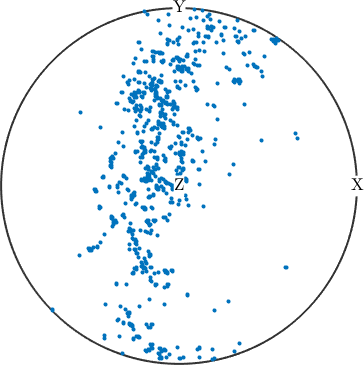

The directions form a narrow, branched band that passes to the left of Z, with smaller isolated clusters near the rim. All directions in this file lie on the upper hemisphere, so 'upper' omits none of them. The option is only a hemisphere filter; it does not identify opposite directions.

A filled contour plot replaces the individual markers with a smoothed estimate of their concentration.

contourf(v,'upper');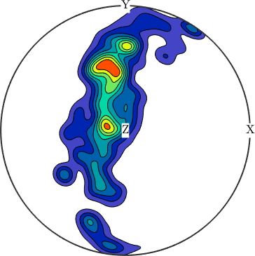

The contour plot separates several maxima within the band. The strongest concentration lies above and left of Z, while the isolated groups remain weaker peaks. These contours are an estimate, not additional measurements, and their shape depends on the smoothing choice.

Spherical Projections explains how the sphere is mapped into these plots. Density Estimation develops the smoothing model and its parameters.

Further Reading

Next

Write directions back to a text file with Export. Turn a long list of observations into a function on the sphere with Density Estimation. Directions attached to a crystal lattice carry crystal symmetry and are represented by Miller indices.

Domain-specific measurements need more information than a vector table. Continue with EBSD Import or Pole Figure Import for those workflows.