Here we describe how to visualize grain boundary properties, e.g., misorientation angle, misorientation axes. Therefore lets start by importing some EBSD data and reconstructing the grain structure.
close all;

% import the data
mtexdata forsterite

% restrict it to a sub-region of interest.
ebsd = ebsd(inpolygon(ebsd,[5 2 10 5]*10^3));

% reconstruct grains
[grains,ebsd.grainId] = calcGrains(ebsd('indexed'),'minPixel',5);

% smooth the grains a bit
grains = smooth(grains,4);
ebsd = EBSD (y↑→x)
Phase Orientations Mineral Color Symmetry Crystal reference frame
0 58485 (24%) notIndexed
1 152345 (62%) Forsterite LightSkyBlue mmm
2 26058 (11%) Enstatite DarkSeaGreen mmm
3 9064 (3.7%) Diopside Goldenrod 12/m1 X||a*, Y||b*, Z||c
Properties: bands, bc, bs, error, mad
Scan unit : um
X x Y x Z : [0, 36550] x [0, 16750] x [0, 0]
Normal vector: (0,0,1)The grain boundary segments of a list of grains are stored within the field
gB = grains.boundarygB = grainBoundary
Segments length mineral 1 mineral 2
869 27592 µm notIndexed Forsterite
36 1562 µm notIndexed Enstatite
42 1361 µm notIndexed Diopside
1398 56197 µm Forsterite Forsterite
654 26372 µm Forsterite Enstatite
522 20750 µm Forsterite Diopside
35 1296 µm Enstatite Enstatite
134 5802 µm Enstatite Diopside
23 951 µm Diopside DiopsideWe may use the plot command to visualize the grain boundaries in the map
% plot phases and grain boundaries
plot(ebsd)
hold on
plot(gB,'lineWidth',2)
hold off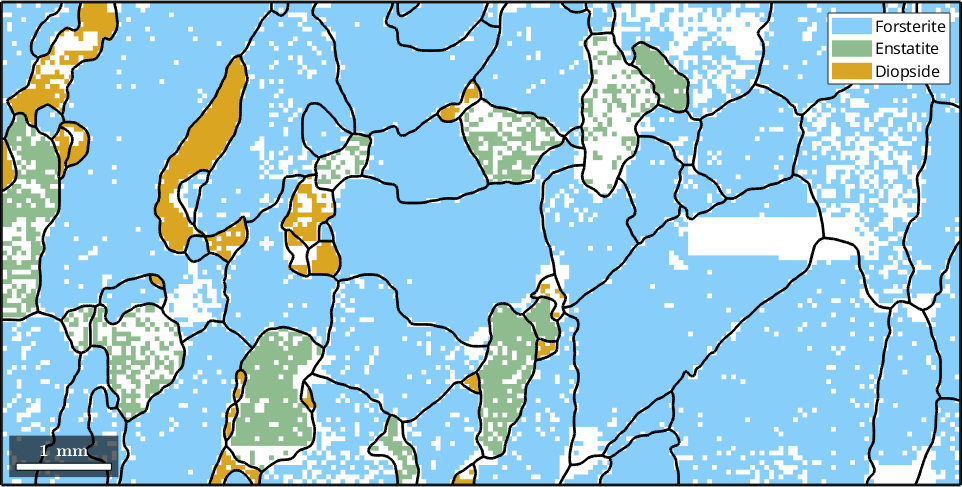
Specific boundaries
Accordingly, we can access the grain boundary of a specific grain by
grains(45).boundary

% lets highlight this specific grain by its boundary
hold on
plot(grains(45).boundary,'lineWidth',4,'lineColor','DarkBlue')
hold off
ans = grainBoundary
Segments length mineral 1 mineral 2
81 3365 µm Forsterite Forsterite
16 720 µm Forsterite Enstatite
9 386 µm Forsterite Diopside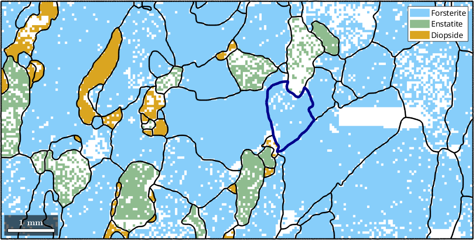
For a multi-phase system, the location of specific phase transitions may be of interest. The following plot highlights all Forsterite to Enstatite phase transitions
hold on
plot(grains.boundary('Fo','En'),'linecolor','DarkGreen','linewidth',4)
hold off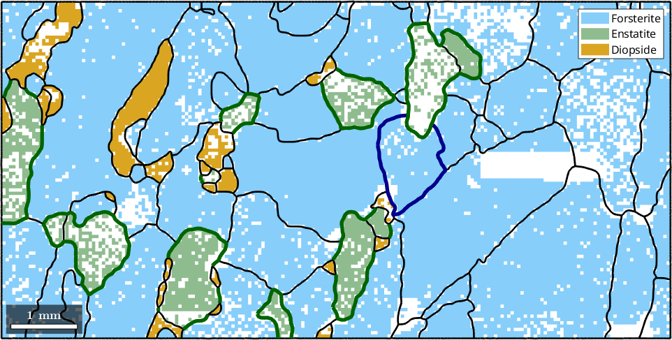
Another type of boundaries is boundaries between measurements that belong to the same grain. This happens if a grain has a texture gradient that loops around these two measurements.
hold on
plot(grains.innerBoundary,'linecolor','red','linewidth',4)
hold off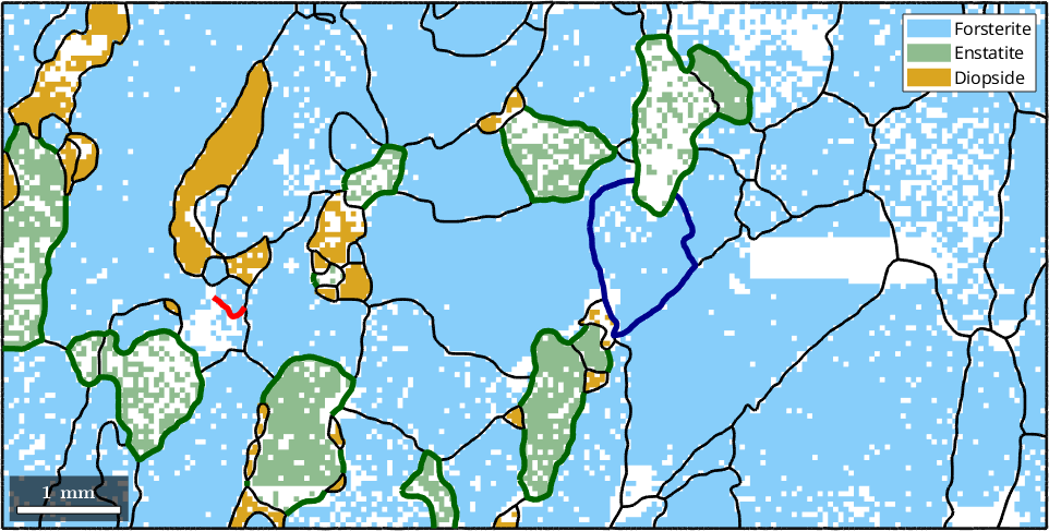
Misorientation angle
The boundary misorientation is the misorientation between the two neighboring pixels of a boundary segment. Depending of the misorientation angle one distinguishes between high angle and low angle grain boundaries. In MTEX we can visualize the boundary misorientation angle by the commands
close all
gB_Fo = grains.boundary('Fo','Fo');
plot(grains,'translucent',1,'micronbar','off')
legend off
hold on
plot(gB_Fo,gB_Fo.misorientation.angle./degree,'linewidth',4)
hold off
mtexColorbar('title','misorientation angle')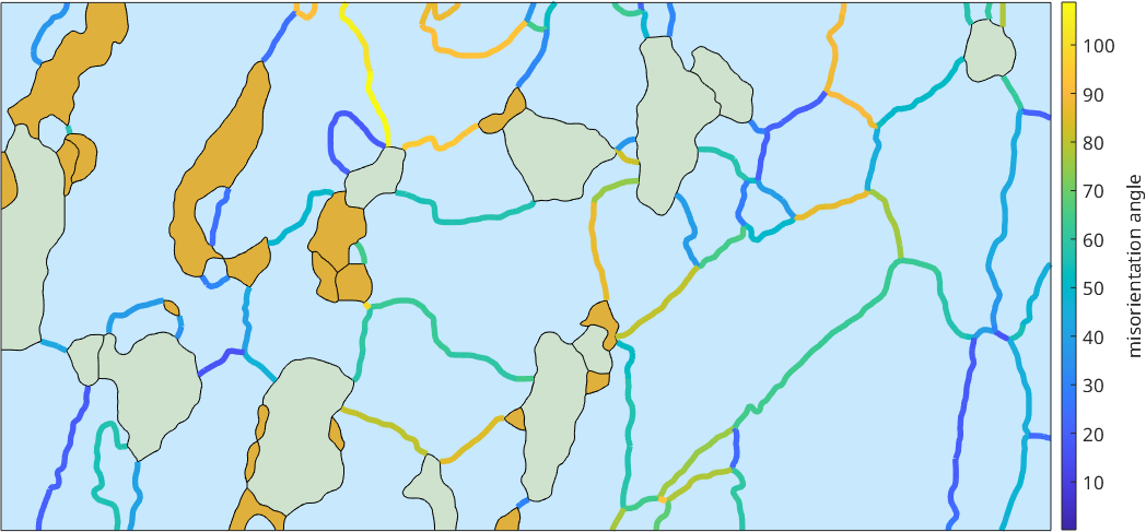
The misorientation axes in crystal coordinates
Similarly as the rotational angle we may colorize the grain boundaries also according the misorientation axes. First of all we have to decide whether we want to visualize the rotational axis in crystal or coordinate system. Second we have to define a color key that translates rotational axes into colors.
Lets start with the rotational axes in crystal coordinates
% computed the axes in specimen coordinates
axes = gB_Fo.misorientation.axis

% define a color key
colorKey = HSVDirectionKey(axes);

% compute colors
color = colorKey.direction2color(axes);

hold on
plot(gB_Fo,'lineColor','black','linewidth',6) % some black background for contrast
plot(gB_Fo,color,'linewidth',4)
hold off
mtexColorbar('visible','off')
axes = Miller (Forsterite)
size: 1398 x 1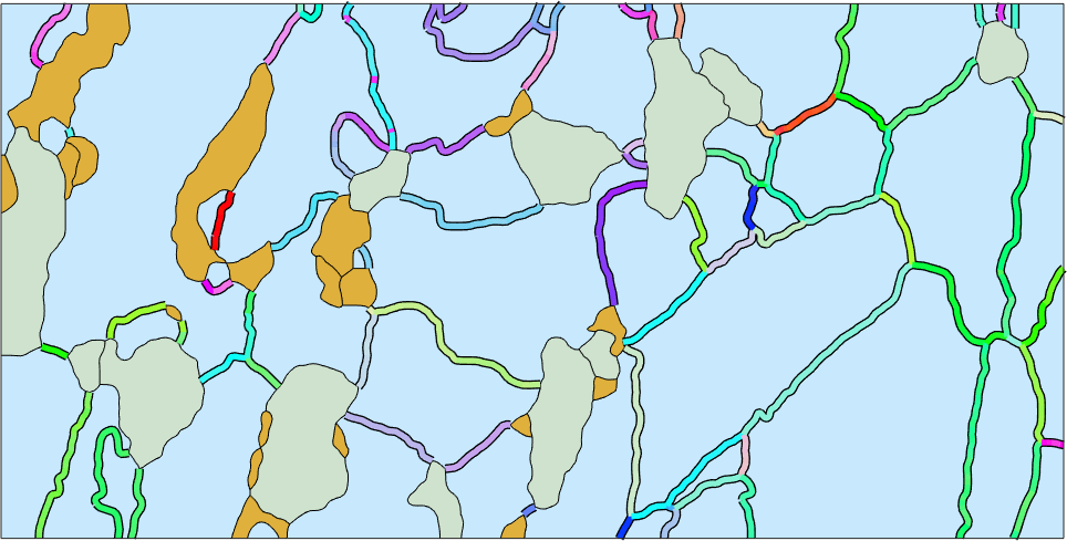
As a colorbar replacement we plot the color key and on top of it the misorientation axes at the grain boundaries
figure(2)
plot(colorKey)
hold on
plot(axes,'MarkerFaceAlpha',0.1,'MarkerEdgeAlpha',0.3,'MarkerColor','black')
hold off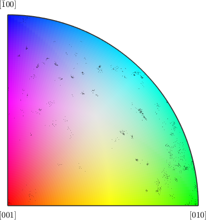
The misorientation axes in specimen coordinates
Analyzing the misorientation axis in specimen coordinates is a bit more involved as it requires to extract the two neighboring orientations to each boundary segment. To do this we use the ebsdId stored in the boundary segments.
figure(1)

% first we reduce the number of boundary segments a bit
% in order to avoid that the plot becomes to messy
gB_red = reduce(gB_Fo,5)

% next we extract for every boundary segment the two orientations at both
% sides
ori = ebsd('id',gB_red.ebsdId).orientations

% the two orientations we use to compute the misorientation axis in
% specimen coordinates
axes = axis(ori(:,1),ori(:,2))

% plot the projection of the misorientation axis on the measurement surface
hold on
quiver(gB_red,axes,'autoScaleFactor',0.4,'color','black')
hold off
gB_red = grainBoundary
Segments length mineral 1 mineral 2
280 11373 µm Forsterite Forsterite
ori = orientation (Forsterite → y↑→x)
size: 280 x 2
axes = vector3d (y↑→x)
size: 280 x 1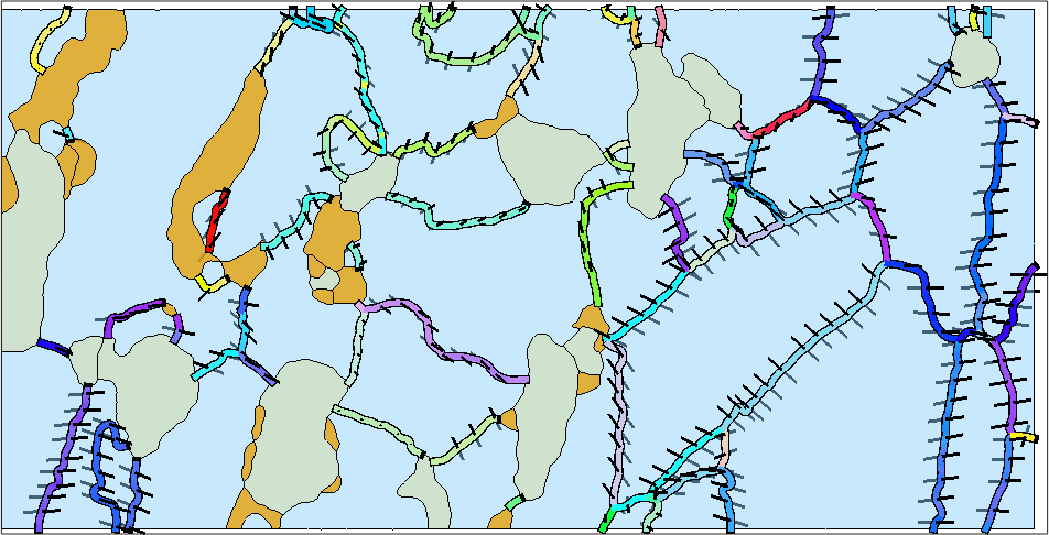
Full Misorientation Colorization
In order to visualize the full misorientation, i.e., axis and angle, one has to define a corresponding color key. One option is the color key described in the paper by S. Patala, J. K. Mason, and C. A. Schuh, Improved representations of misorientation information for grain boundary, Prog. Mater. Sci., vol. 57, no. 8, pp. 1383-1425, 2012.
% plot the grains
close all
plot(grains,'micronbar','off')
legend off

% define the color key
colorKey = PatalaColorKey(gB_Fo);

hold on
plot(gB_Fo,'linewidth',7)
hold on
color = colorKey.orientation2color(gB_Fo.misorientation);
plot(gB_Fo,squeeze(color),'linewidth',4)
hold off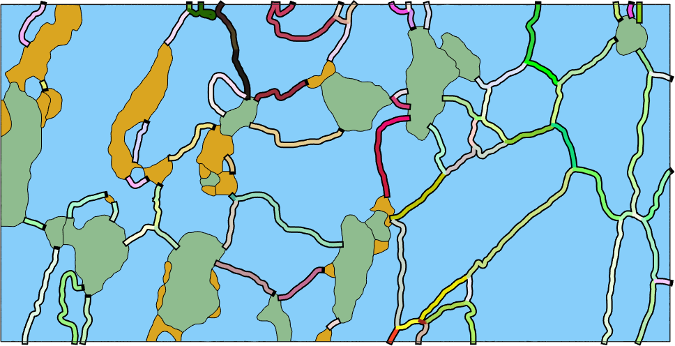
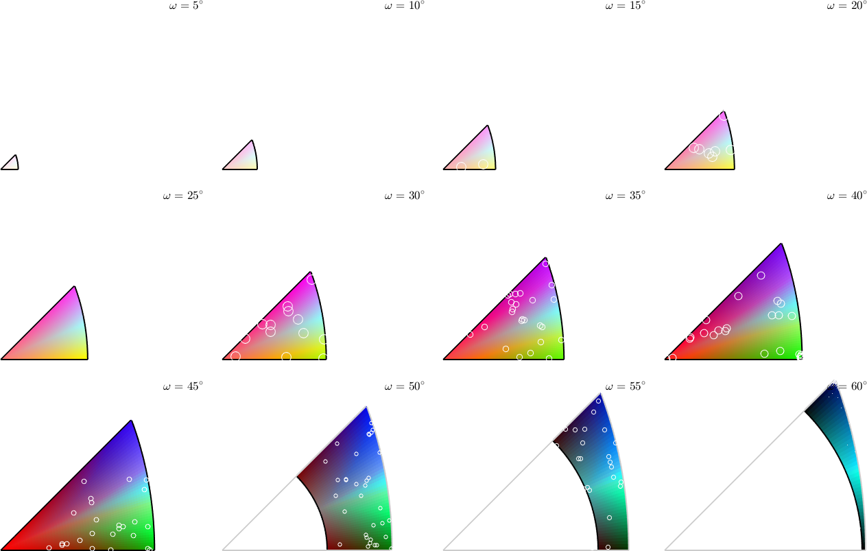
Lets visualize the color key as axis angle sections through the misorientation space
figure(2)
plot(colorKey,'layout',[3,4])

% and plot the misorienations on top
plot(gB_Fo.misorientation,...
  'MarkerFacecolor','none','add2all','MarkerSize',4)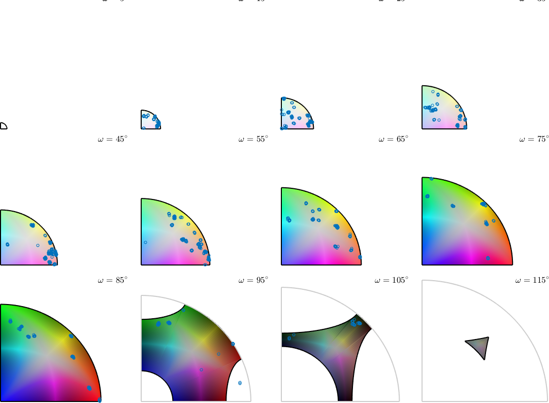
Lets illustrate this color coding also at a iron sample.
% import the data
mtexdata csl

% grain segmentation and smoothing
[grains,ebsd.grainId] = calcGrains(ebsd('indexed'));
grains = smooth(grains,2);
gB = grains.boundary('iron','iron');

% and plot image quality + orientation
close all
plot(ebsd,log(ebsd.prop.iq),'figSize','large')
mtexColorMap black2white
setColorRange([.5,5])
hold on
plot(grains,grains.meanOrientation,'FaceAlpha',0.4)

% define the color key and colorize the grain boundaries
colorKey = PatalaColorKey(gB)
color = colorKey.orientation2color(gB.misorientation);
hold on
plot(gB,squeeze(color),'linewidth',4,'smooth')
hold off
ebsd = EBSD (y↑→x)
Phase Orientations Mineral Color Symmetry Crystal reference frame
0 5 (0.0032%) notIndexed
-1 154107 (100%) iron LightSkyBlue m-3m
Properties: ci, error, iq
Scan unit : um
X x Y x Z : [0, 511] x [0, 300] x [0, 0]
Normal vector: (0,0,1)
colorKey =
PatalaColorKey with properties:
CS1: [1×1 crystalSymmetry]
CS2: [1×1 crystalSymmetry]
antipodal: 1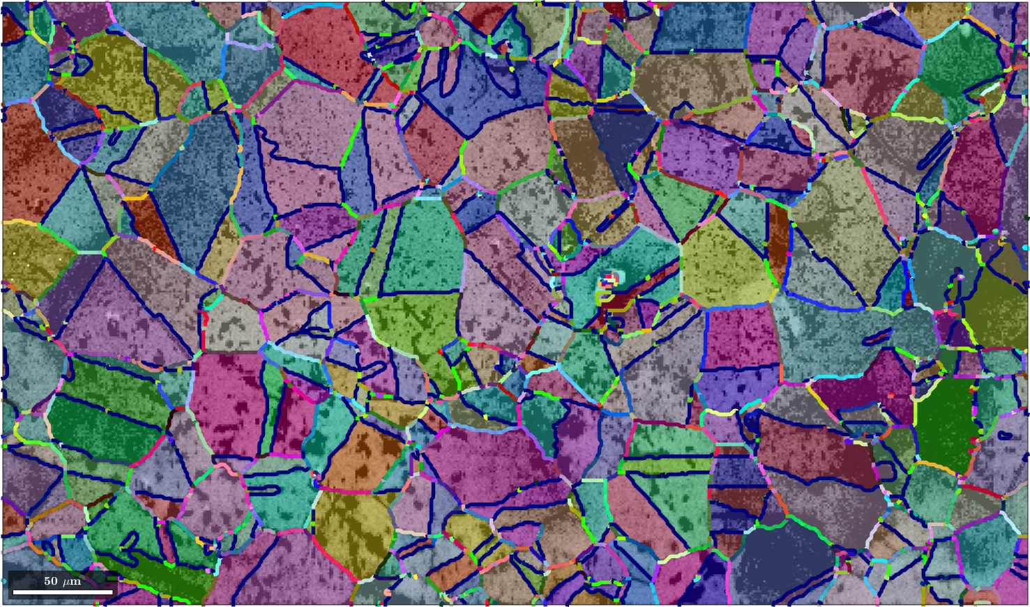
At the end we plot the colorized misorientation space in axis angle sections. Note that in this plot misorientations mori and inv(mori) are associated.
plot(colorKey,'axisAngle',(5:5:60)*degree,'layout',[3,4])

plot(gB.misorientation,'points',300,'add2all',...
  'MarkerFaceColor','none','MarkerEdgeColor','w')
plotting 300 random orientations out of 20356 given orientations