Spherical Harmonics

Spherical harmonics are standard wave-like functions on the unit sphere. They play the same role for a spherical function that sines and cosines play for a periodic signal. Low degrees describe broad variation, while higher degrees can describe progressively finer angular detail.

MTEX uses spherical harmonics as an orthonormal basis for square-integrable functions on the sphere. The preceding Harmonic Representation page explains how an S2FunHarmonic stores and combines their coefficients. This page examines the basis functions themselves.

plottingConvention.default('y↑→x');
close all

Evaluate all orders of one degree

A spherical harmonic is identified by its degree \(m\) and its order \(l\). For a fixed degree \(m\), the order runs from \(-m\) to \(m\). sphericalY evaluates all \(2m+1\) orders at once and returns them in ascending order.

Here the evaluation direction is the specimen X direction. The three entries are \(Y_1^{-1}(\mathbf{x})\), \(Y_1^0(\mathbf{x})\), and \(Y_1^1(\mathbf{x})\).

v = vector3d.X
Y1AtX = sphericalY(1,v)

v = vector3d (y↑→x)
  x y z
  1 0 0
Y1AtX =
    0.3455    0.0000    0.3455

Read the degree-one values

The two outer entries are equal at this direction. The middle entry is zero up to floating-point round-off. Changing v evaluates the same three basis functions at another direction on the sphere.

Select one basis function by its coefficient

The coefficient vector of an S2FunHarmonic is ordered degree by degree. Degree zero occupies the first entry. The three degree-one entries then correspond to orders \(-1\), 0, and 1. A one in the fourth position therefore selects \(Y_1^1\).

Y = S2FunHarmonic([0;0;0;1])
valueFromSeries = Y.eval(v)

Y = S2FunHarmonic (y↑→x)
  bandwidth: 1
  isReal: false
 
valueFromSeries =
    0.3455

Compare the two evaluation routes

valueFromSeries equals the last entry of Y1AtX. Use sphericalY when the basis values themselves are required. Use S2FunHarmonic when coefficients will be combined, rotated, differentiated, or integrated.

Check the MTEX normalization

Several normalizations of spherical harmonics are common in the literature. MTEX normalizes every basis function to unit \(L^2\) norm. The selected basis function therefore has norm one.

normOfY = norm(Y)

normOfY =
     1

See the first ten basis functions

The identity matrix selects one coefficient in each column. The command below therefore plots the first ten spherical harmonics in MTEX coefficient order.

basis = S2FunHarmonic(eye(10));
surf(basis,'layout',[2,5],'figSize','large')

mtexFig = gcm;
basisNames = {'\(Y_0^0\)','\(Y_1^{-1}\)','\(Y_1^0\)','\(Y_1^1\)', ...
  '\(Y_2^{-2}\)','\(Y_2^{-1}\)','\(Y_2^0\)','\(Y_2^1\)','\(Y_2^2\)', ...
  '\(Y_3^{-3}\)'};
for k = 1:numel(basisNames)
  mtexTitle(mtexFig.children(k),basisNames{k});
end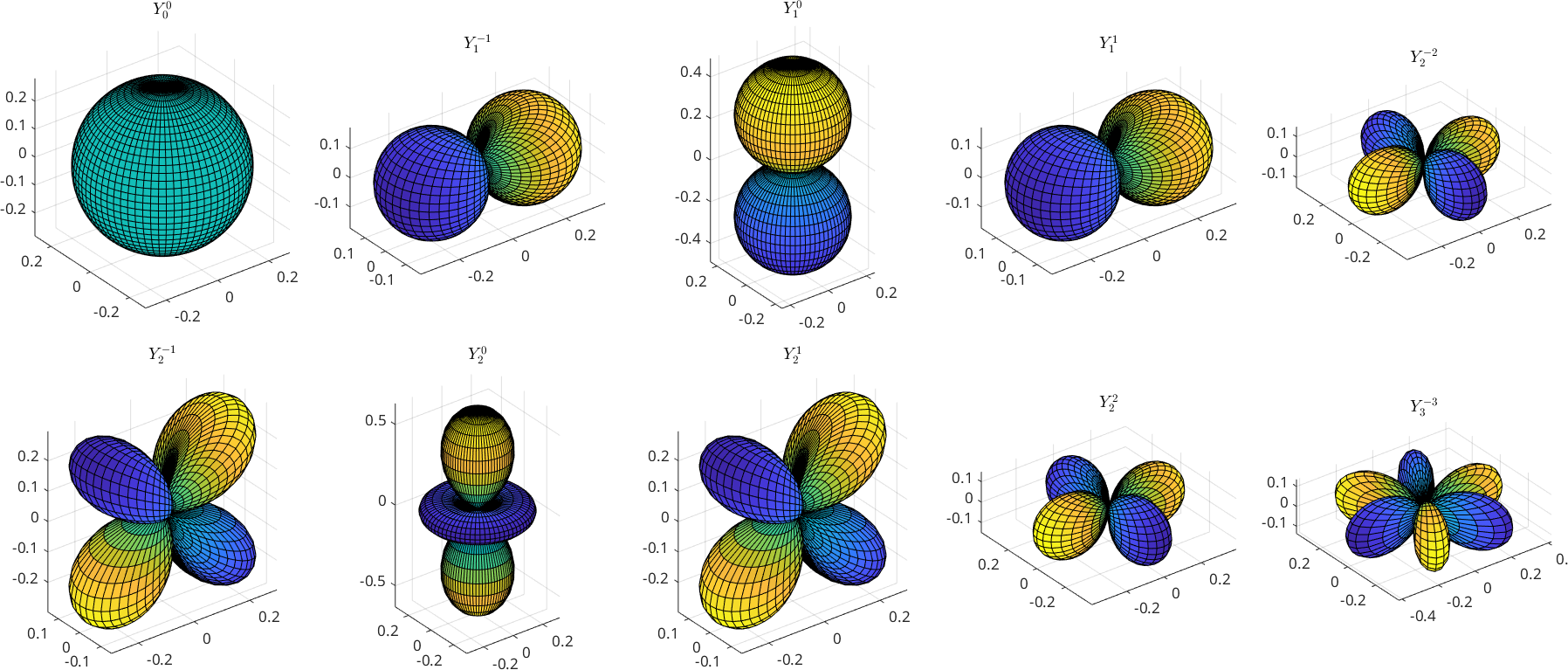

Read the basis plot

The constant degree-zero function is the sphere in the first panel. Degree one has one broad pair of lobes. Degree two changes sign more often, and the first degree-three function begins an even finer pattern. Radius shows magnitude, while colour distinguishes the signed real part. The complex orders are displayed through the real part used by surf.

The maths behind the basis

Write a point on the sphere in polar coordinates as

\[ \mathbf{\xi}=(\sin\theta\cos\rho,\sin\theta\sin\rho,\cos\theta). \]

In the MTEX convention, the spherical harmonic of degree \(m\) and nonnegative order \(l=0,\ldots,m\) is

\[ Y_m^l(\mathbf{\xi}) = \sqrt{\frac{2m+1}{4\pi}}\, P_m^{l}(\cos\theta)\,\mathrm e^{\mathrm i l\rho}. \]

Negative orders are completed by \(Y_m^{-l}(\mathbf{\xi})=\overline{Y_m^l(\mathbf{\xi})}\). The associated Legendre functions are

\[ P_m^l(x) = \sqrt{\frac{(m-l)!}{(m+l)!}}\, (1-x^2)^{l/2}\frac{\mathrm d^l}{\mathrm d x^l}P_m(x), \]

where \(m\in\mathbf{N}_0\). The Legendre polynomials follow Rodrigues' formula

\[ P_m(x)=\frac{1}{2^m m!}\frac{\mathrm d^m}{\mathrm d x^m} (x^2-1)^m. \]

The spherical harmonics form an orthonormal basis in \(L^2(\mathbb{S}^2)\). MTEX defines the norm by

\[ \|f\|_2=\left(\int_{\mathbb{S}^2}|f(\mathbf{\xi})|^2\, \mathrm d\mathbf{\xi}\right)^{1/2}. \]

Consequently, \(\|1\|_2^2=4\pi\) and \(\|Y_m^l\|_2=1\) for every \(m\) and \(l\). See Integration and norms for integration of spherical functions.

References

Next

Continue with Fourier Series to see how the same degree-and-order bookkeeping reduces to ordinary Fourier modes on the circle.

References

- J. R. Driscoll and D. M. Healy, Computing Fourier transforms and convolutions on the 2-sphere, Advances in Applied Mathematics 15 (1994), 202--250, develops orthonormal spherical harmonic expansions and their fast transforms.