Parent Child Variants

Parent Child Variants edit page

The crystallographic structure of most materials is depended on external conditions as temperature and pressure. When the external conditions change the crystals may undergo a phase transition from the initial phase, often called parent phase, into the child phase. While both phases still have the same chemical composition their crystallographic structure might be quite different. A typical example are the alpha and beta phase of titanium. While the parent beta phase is cubic

csBeta = crystalSymmetry('432',[3.3 3.3 3.3],'mineral','Ti (beta)');

the child alpha phase is hexagonal

csAlpha = crystalSymmetry('622',[3 3 4.7],'mineral','Ti (alpha)');

Let oriParent

oriParent = orientation.rand(csBeta);

be the orientation of the atomic lattice before phase transition and oriChild the orientation of the atomic lattice after the phase transition. Since during a phase transition the atoms reorder with respect to a minimal energy constraint, both orientations oriParent and oriChild are in a specific orientation relationship with respect to each other. In the case of alpha and beta Titanium the dominant orientation relationship is described by the Burger orientation relationship

beta2alpha = orientation.Burgers(csBeta,csAlpha)

beta2alpha = misorientation (Ti (beta) → Ti (alpha))
 
 (110) || (0001)   [1-11] || [-2110]

A corresponding child orientation would then be

oriChild = oriParent * inv(beta2alpha)

oriChild = orientation (Ti (alpha) → xyz)
 
  Bunge Euler angles in degree
     phi1     Phi    phi2
  261.104 66.2529 236.292

This orientation relationship is characterized by alignment of hexagonal (0001) plane with the cubic (110) plane and alignment of the hexagonal [2-1-10] direction with the cubic [-11-1] direction.

% (110) / (0001) pole figure
plotPDF(oriParent,Miller(1,1,0,csBeta),...
  'MarkerSize',20,'MarkerFaceColor','none','linewidth',4)
hold on
plot(oriChild.symmetrise * Miller(0,0,0,1,csAlpha),'MarkerSize',12)
xlabel(char(Miller(0,0,0,1,csAlpha)),'color',ind2color(2))
hold off

% [111] / [2-1-10] pole figure
nextAxis(2)
plotPDF(oriParent,Miller(1,1,1,csBeta,'uvw'),'upper',...
  'MarkerSize',20,'MarkerFaceColor','none','linewidth',4)

dAlpha = Miller(2,-1,-1,0,csAlpha,'uvw');
hold on
plot(oriChild.symmetrise * dAlpha,'MarkerSize',12)
xlabel(char(dAlpha),'color',ind2color(2))
hold off
drawNow(gcm)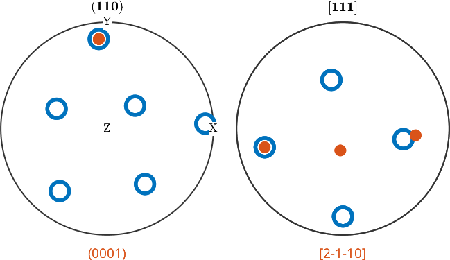

We could also use these alignment rules to define the orientation relationship as

beta2alpha = orientation.map(Miller(1,1,0,csBeta),Miller(0,0,0,1,csAlpha),...
      Miller(-1,1,-1,csBeta),Miller(2,-1,-1,0,csAlpha));

The advantage of the above definition by the alignment of different crystal directions is that it is independent of the convention used for the hexagonal crystal coordinate system.

Child Variants

Due to crystal symmetry each orientation of a parent beta grain has 24 different may transform into up to 24 child orientations.

oriParentSym = oriParent.symmetrise

oriParentSym = orientation (Ti (beta) → xyz)
  size: 24 x 1

Applying the beta2alpha phase relationship to these 24 different representations we obtain 24 child orientations.

oriChild = oriParentSym * inv(beta2alpha)

oriChild = orientation (Ti (alpha) → xyz)
  size: 24 x 1

Some of these child orientations are symmetrically equivalent with respect to the hexagonal child symmetry. In fact there are 12 pairs of symmetrically equivalent child orientations as depicted in the following inverse pole figure.

plotIPDF(oriChild,vector3d.Z)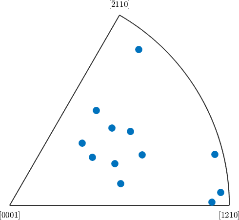

These 12 pairs are called the variants of the parent orientation oriParent with respect to the orientation relation ship beta2alpha. They can be computed more directly using the command variants.

oriChild = variants(beta2alpha,oriParent);

for i = 1:12
  plotIPDF(oriChild(i),ind2color(i),vector3d.Z,'label',i,'MarkerEdgeColor','k');
  hold on
end
hold off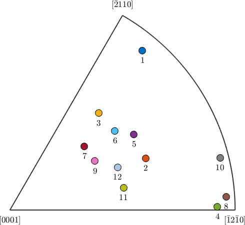

As we can see each variant can be associated by a variantId. You can pick specific variants by their variantId using the syntax

oriChild = variants(beta2alpha,oriParent,2:3)

oriChild = orientation (Ti (alpha) → xyz)
  size: 1 x 2
 
  Bunge Euler angles in degree
     phi1     Phi    phi2
  11.8095 155.789 128.635
  27.7322 36.4051 312.007

It is important to understand that the reduction to 12 variants from 24 symmetrically equivalent parent orientations comes from the specific Burger orientation relationship. For a general orientation relationship, e.g., if we disturb the OR a little bit

beta2alpha = beta2alpha .* orientation.rand(csBeta,csBeta,'maxAngle',2*degree)

beta2alpha = misorientation (Ti (beta) → Ti (alpha))
 
  Bunge Euler angles in degree
     phi1     Phi    phi2
  185.268 88.0499 45.4066

we will always have exactly 24 variants. For the above example we observe how the 12 pairs of orientations which diverge slightly.

plotIPDF(variants(beta2alpha,oriParent),vector3d.Z)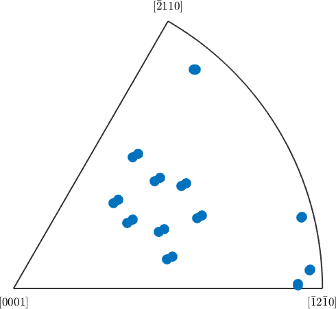

Sometimes one faces the inverse question, i.e., determine the variantId from a parent and a child orientation or a pair of child orientations. This can be done using the command calcVariants which is discussed in detail in the section parent grain reconstruction.

Parent Variants

TODO