Ghost Effect Analysis

A general problem in estimating an ODF from pole figure data is the fact that the odd order Fourier coefficients of the ODF are not present anymore in the pole figure data and therefore it is difficult to estimate them. Artifacts in the estimated ODF that are due to underestimated odd order Fourier coefficients are called ghost effects. It is known that for sharp textures the ghost effect is relatively small due to the strict non-negativity condition. For weak textures, however, the ghost effect might be remarkable. For those cases, MTEX provides the option ghost_correction which tries to determine the uniform portion of the unknown ODF and to transform the unknown weak ODF into a sharp ODF by substracting this uniform portion. This is almost the approach Matthies proposed in his book (He called the uniform portion phon). In this section, we are going to demonstrate the power of ghost correction at a simple, synthetic example.

Construct Model ODF

A unimodal ODF with a high uniform portion.

cs = crystalSymmetry('222');
mod1 = orientation.byEuler(0,0,0,cs);
odf = 0.9*uniformODF(cs) + ...
  0.1*unimodalODF(mod1,'halfwidth',10*degree)

odf = SO3FunRBF (222 → xyz)
 
  <strong>uniform component</strong>
  weight: 0.9
 
  <strong>unimodal component</strong>
  kernel: de la Vallee Poussin, halfwidth 10°
  center: 1 orientations
 
  Bunge Euler angles in degree
  phi1    Phi   phi2 weight
     0      0      0    0.1

Simulate pole figures

% specimen directions
r = equispacedS2Grid('resolution',5*degree,'antipodal');

% crystal directions
h = Miller({1,0,0},{0,1,0},{0,0,1},cs);

% compute pole figures
pf = calcPoleFigure(odf,h,r);

plot(pf)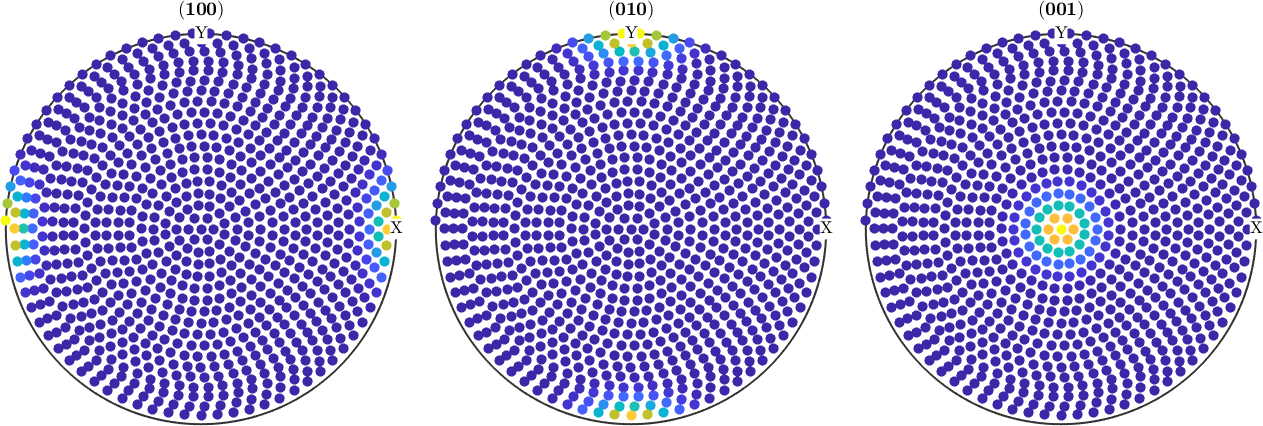

ODF Estimation

without ghost correction:

rec = calcODF(pf,'noGhostCorrection','silent');

with ghost correction:

rec_cor = calcODF(pf,'silent');

Compare RP Errors

without ghost correction:

calcError(pf,rec,'RP')

ans =
    0.0089    0.0088    0.0106

with ghost correction:

calcError(pf,rec_cor,'RP')

ans =
    0.0262    0.0250    0.0265

Compare Reconstruction Errors

without ghost correction:

calcError(rec,odf)

ans =
    0.1253

with ghost correction:

calcError(rec_cor,odf)

ans =
    0.0055

Plot the ODFs

without ghost correction:

plot(rec,'sections',9,'silent','sigma')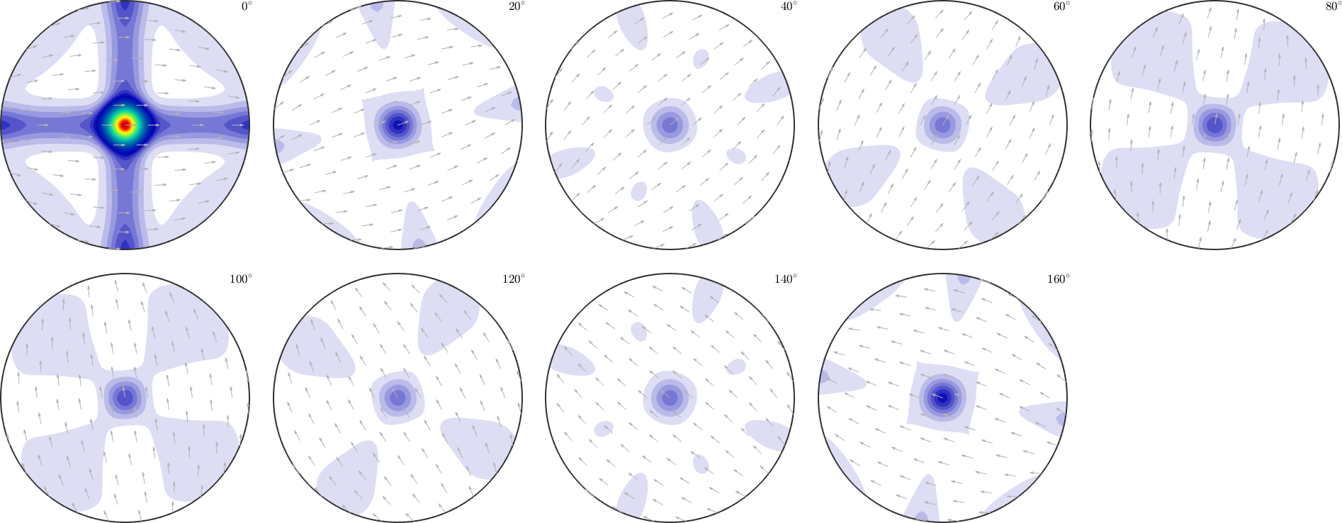

with ghost correction:

plot(rec_cor,'sections',9,'silent','sigma')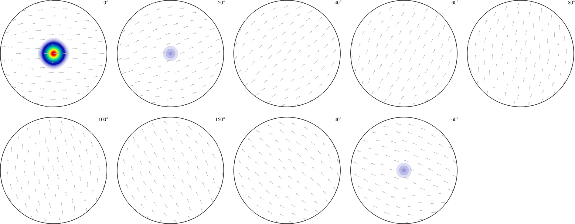

radial plot of the true ODF

close all
f = fibre(Miller(0,1,0,cs),yvector);
plot(odf,f,'linewidth',2);
hold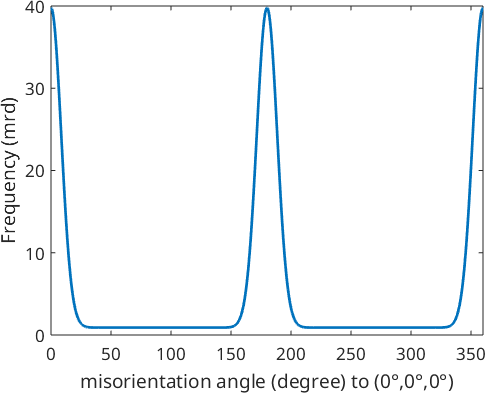 all

radial plot without ghost correction:

plot(rec,f,'linewidth',2);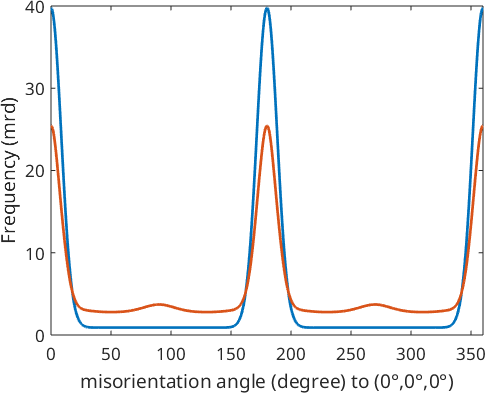

radial plot with ghost correction:

plot(rec_cor,f,'linestyle','--','linewidth',2);
hold off
legend({'true ODF','without ghost correction','with ghost correction'})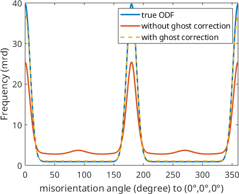

Calculate Fourier coefficients

Next, we want to analyze the fit of the Fourier coefficients of the reconstructed ODFs. To this end, we first compute Fourier representations for each ODF

odf = FourierODF(odf,25)
rec = FourierODF(rec,25)
rec_cor = FourierODF(rec_cor,25)

odf = SO3FunHarmonic (222 → xyz)
  bandwidth: 25
  weight: 1
 
 
rec = SO3FunHarmonic (222 → xyz)
  bandwidth: 48
  weight: 1
 
 
rec_cor = SO3FunHarmonic (222 → xyz)
  bandwidth: 48
  weight: 1

Calculate Reconstruction Errors from Fourier Coefficients

without ghost correction:

calcError(rec,odf,'L2')

ans =
    0.3592

with ghost correction:

calcError(rec_cor,odf,'L2')

ans =
    0.0326

Plot Fourier Coefficients

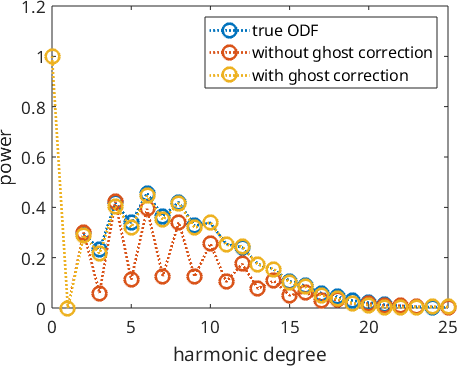
Plotting the Fourier coefficients of the recalculated ODFs shows that the Fourier coefficients without ghost correction oscillates much more than the Fourier coefficients with ghost correction

true ODF

close all;
plotSpektra(odf,'linewidth',2)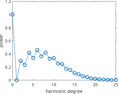

keep plotting windows and add next plots

hold all

Without ghost correction:

plotSpektra(rec,'linewidth',2)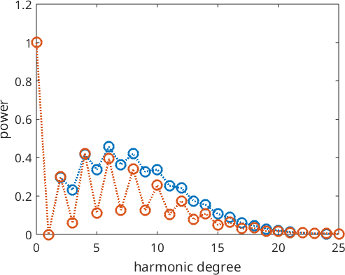

with ghost correction

plotSpektra(rec_cor,'linewidth',2)
legend({'true ODF','without ghost correction','with ghost correction'})
% next plot command overwrites plot window
hold off