ODF Estimation from EBSD data

In order to discuss ODF estimation from individual orientation data we start by loading an EBSD data set

mtexdata copper

plot(ebsd,ebsd.orientations)

ebsd = EBSD (y↑→x)
 
 Phase  Orientations  Mineral         Color  Symmetry  Crystal reference frame
     0  16116 (100%)   Copper  LightSkyBlue       432                         
 
 Properties: confidenceindex, fit, imagequality, semsignal, unknown_11, unknown_12, unknown_13, unknown_14
 Scan unit : um
 X x Y x Z : [0, 590] x [0, 585] x [0, 0]
 Normal vector: (0,0,1)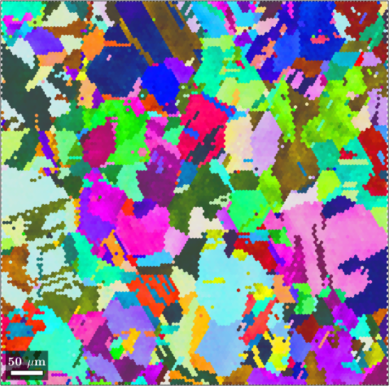

of copper. The orientation distribution function can now be computed by

odf = calcDensity(ebsd('copper').orientations)

plotSection(odf,'contourf')
mtexColorMap LaboTeX
mtexColorbar

odf = SO3FunHarmonic (Copper → y↑→x)
  bandwidth: 25
  weight: 1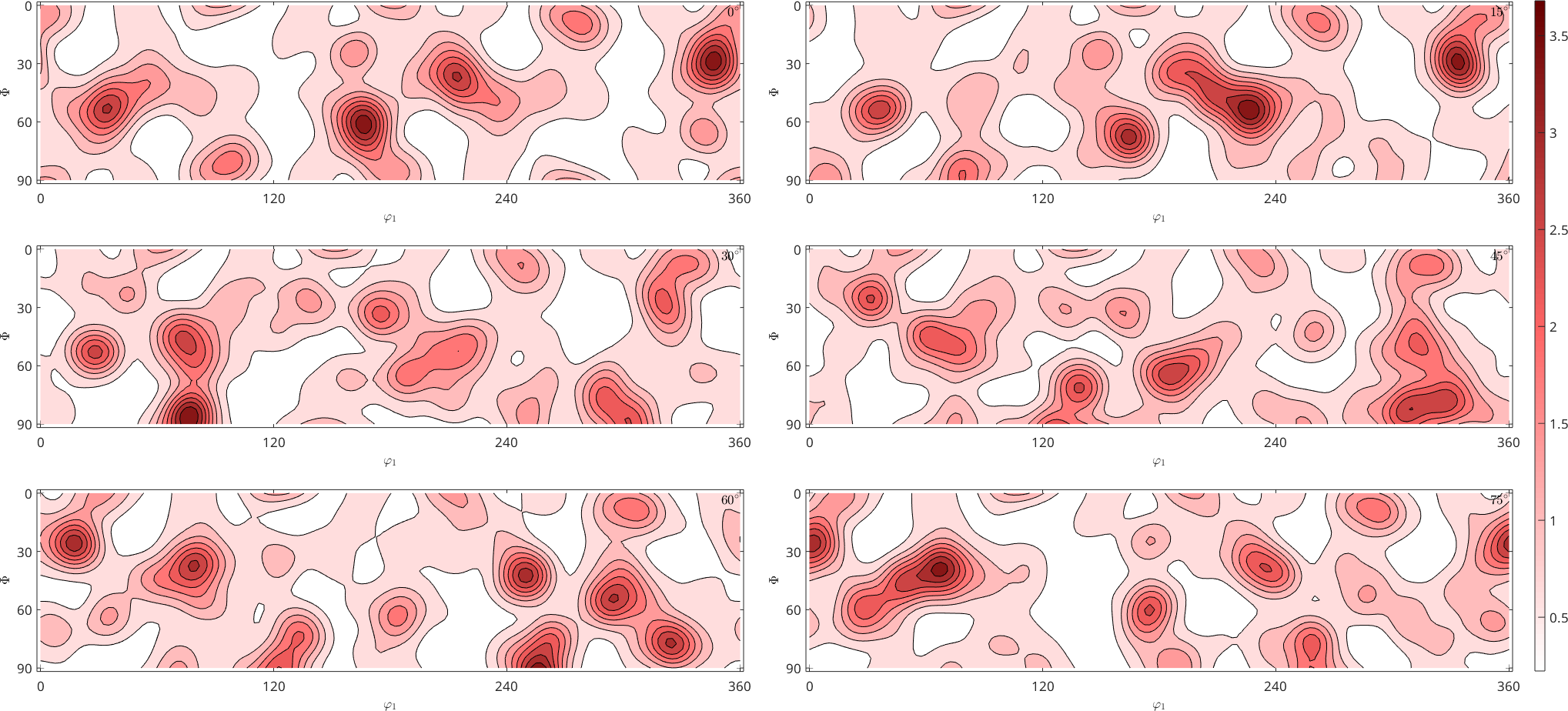

The function calcDensity implements the ODF estimation from EBSD data in MTEX. The underlying statistical method is called kernel density estimation, which can be seen as a generalized histogram. To be more precise, let's \(\psi : SO(3) \to R\) be a radially symmetric, unimodal model ODF. Then the kernel density estimator for the individual orientation data \(o_1,o_2,\ldots,o_M\) is defined as

\[f(o) = \frac{1}{M} \sum_{i=1}^{M} \psi(o o_i^{-1})\]

The choice of the model ODF \(\psi\) and in particular its halfwidth has a great impact in the resulting ODF. If no halfwidth is specified the default halfwidth of 10 degrees is selected.

Automatic halfwidth selection

MTEX includes an automatic halfwidth selection algorithm which is called by the command calcKernel. To work properly, this algorithm needs spatially independent EBSD data as in the case of this dataset of very rough EBSD measurements (only one measurement per grain).

% try to compute an optimal kernel
psi = calcKernel(ebsd.orientations)

psi = SO3DeLaValleePoussinKernel
  bandwidth: 84
  halfwidth: 2.7°

In the above example, the EBSD measurements are spatial dependent and the resulting halfwidth is too small. To avoid this problem we have to perform grain reconstruction first and then estimate the halfwidth from the grains.

% grains reconstruction
grains = calcGrains(ebsd,'minPixel',5);

% compute optimal halfwidth from the meanorientation of grains
psi = calcKernel(grains('co').meanOrientation)

% compute the ODF with the kernel psi
odf = calcDensity(ebsd('co').orientations,'kernel',psi)

psi = SO3DeLaValleePoussinKernel
  bandwidth: 51
  halfwidth: 4.7°
 
 
odf = SO3FunHarmonic (Copper → y↑→x)
  bandwidth: 51
  weight: 1

Once an ODF is estimated all the functionality MTEX offers for ODF analysis and ODF visualization is available.

h = [Miller(1,0,0,odf.CS),Miller(1,1,0,odf.CS),Miller(1,1,1,odf.CS)];
plotPDF(odf,h,'antipodal','silent')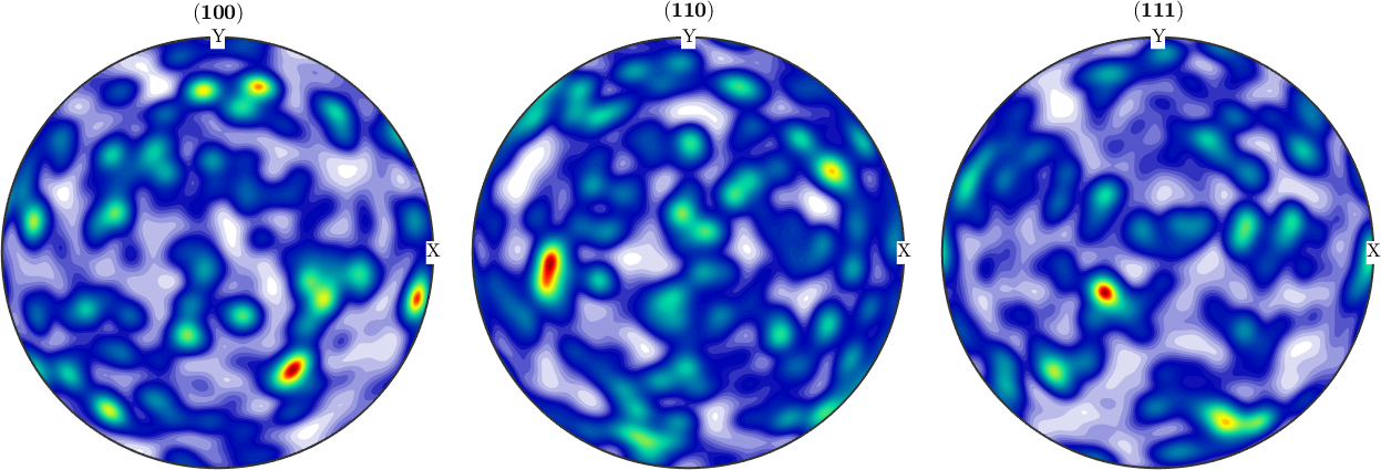

Effect of halfwidth selection

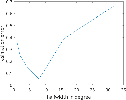
As mentioned above a proper halfwidth selection is crucial for ODF estimation. The following simple numerical experiment illustrates the dependency between the kernel halfwidth and the estimated error.

Let's start with a model ODF and simulate some individual orientation data.

modelODF = fibreODF(Miller(1,1,1,crystalSymmetry('cubic')),xvector);
ori = discreteSample(modelODF,10000)

ori = orientation (m-3m → y↑→x)
  size: 10000 x 1

Next we define a list of kernel halfwidth ,

hw = [1*degree, 2*degree, 4*degree, 8*degree, 16*degree, 32*degree];

estimate for each halfwidth an ODF and compare it to the original ODF.

e = zeros(size(hw));
for i = 1:length(hw)

  odf = calcDensity(ori,'halfwidth',hw(i),'silent');
  e(i) = calcError(modelODF, odf);

end

After visualizing the estimation error we observe that its value is large either if we choose a very small or a very large halfwidth. In this specific example, the optimal halfwidth seems to be about 4 degrees.

close all
plot(hw/degree,e)
xlabel('halfwidth in degree')
ylabel('esimation error')