In MTEX, one can calculate with three dimensional directions as with ordinary numbers, i.e. we can use the predefined vectors vector3d.X, vector3d.Y, and vector3d.Z and set
v = vector3d.X + 2*vector3d.Yv = vector3d (y↑→x)
x y z
1 2 0Moreover, all basic vector operations as "+", "-", "*", inner product, cross product are implemented in MTEX.
u = dot(v,vector3d.Y) * vector3d.Y + 2 * cross(v,vector3d.Z)u = vector3d (y↑→x)
x y z
4 0 0Besides the standard linear algebra operations, there are also the following functions available in MTEX.
|
angle between two specimen directions |
|
|
inner product |
|
|
cross product |
|
|
length of the specimen directions |
|
|
normalize length to 1 |
|
|
sum over all specimen directions in v |
|
|
mean over all specimen directions in v |
|
|
conversion to spherical coordinates |
A simple example for applying the norm function is to normalize a set of specimen directions
u = u ./ norm(u)u = vector3d (y↑→x)
x y z
1 0 0Lists of vectors
As any other MTEX variable you can combine several vectors to a list of vectors. Additionally, all the operators operations mentioned before will work elementwise on a list of vectors. See Working with lists on how to manipulate lists in Matlab.
Using the brackets v = [v1,v2] two lists of vectors can be joined to a single list. Now each single vector is accesable via v(1) and v(2).
w = [v,u];
w(1)
w(2)
ans = vector3d (y↑→x)
x y z
1 2 0
ans = vector3d (y↑→x)
x y z
1 0 0When calculating with concatenated specimen directions all operations are performed componentwise for each specimen direction.
w = w + v;A list of vectors can be indexed directly by specifying the ids of the vectors one is interested in, e.g.
% import many vectors from a file
fname = fullfile(mtexDataPath,'vector3d','vectors.txt');
v = vector3d.load(fname,'ColumnNames',{'polar angle','azimuth angle'})

% extract vectors 1 to 5
v(1:5)
v = vector3d (y↑→x)
size: 1000 x 1
ans = vector3d (y↑→x)
size: 5 x 1
x y z
0.174 0.984 0.0454
0.00906 0.822 0.569
0.43 0.901 0.0587
-0.447 0.0187 0.894
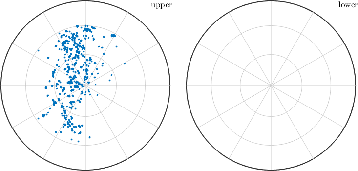
-0.14 0.556 0.82gives the first 5 vectors from the list, or by logical indexing. The following command plots all vectors with an polar angle smaller then 60 degree
scatter(v(v.theta<60*degree),'grid','on')