Import Pole Figure Data

Importing pole figure data in MTEX means to create a PoleFigure object from data files containing diffraction data. Once such an object has been created the data can be analyzed and processed in many ways. Furthermore, such a PoleFigure object is the starting point for PoleFigure to ODF estimation.

Importing pole figure data using the import wizard

The import wizard can be started either by typing into the command line

import_wizard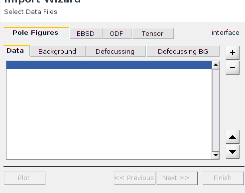

or by using the start menu item Start/Toolboxes/MTEX/Import Wizard. Pole figure data can be also imported via the file browser by choosing Import Data from the context menu of the selected file if its file extension was previously registered with the mtex_settings.m

The import wizard guides through the correct setup of:

In the end, the imported wizard creates a workspace variable or generates a m-file loading the data automatically. Furthermore appending a template script allows radip data processing.

Supported Data Formats

The import wizard currently supports following pole figure formats:

See PoleFigure.load for further information or follow the hyperlinks of the table above for an example.

If the interface is not automatically recognized, but the data has the form of an ASCII list:

polar_1 azimuthal_1 intensity_1
polar_2 azimuthal_2 intensity_2
polar_3 azimuthal_3 intensity_3
.       .           .
.       .           .
.       .           .
polar_n azimuthal_n intensity_n

an additional tool asks you to associate the columns with the corresponding property. See also loadPoleFigure_generic, which provides an easy way to import diffraction data from such an ASCII list. The list may contain an arbitrary number of header lines, columns or comments and the actual order of the columns may be specified by options.

If you have any comments, remarks or request on interfaces please contact us.

The Import Script

Diffraction data stored in one of the formats above can also be imported using the command PoleFigure.load. It automatically detects the data format and imports the data. In dependency of the data format, it might be necessary to specify the Miller indices and the structure coefficients. The general syntax is

An import script generated by the import wizard has the following form:

cs = crystalSymmetry('32',[1.4,1.4,1.5]); % crystal symmetry

% location of the data files
fnames = {...
  fullfile(mtexDataPath,'PoleFigure','dubna','Q(10-10)_amp.cnv'),...
  fullfile(mtexDataPath,'PoleFigure','dubna','Q(10-11)(01-11)_amp.cnv')};

% crystal directions
h = {Miller(1,0,-1,0,cs),[Miller(0,1,-1,1,cs),Miller(1,0,-1,1,cs)]};

% structure coefficients
c = {1,[0.52 ,1.23]};

% load data
pf = PoleFigure.load(fnames,h,cs,'superposition',c)

pf = PoleFigure (xyz)
  crystal symmetry : 321, X||a*, Y||b, Z||c*
 
  h = (10-10), r = 72 x 19 points
  h = (01-11)(10-11), r = 72 x 19 points

Once such a import script for pole figure data has been created, it can be easily modified and extend, e.g.:

% plot the data
plot(pf)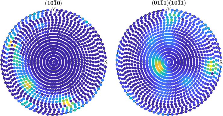

Writing your own interface

MTEX also provides a way to import data from formats currently not supported directly. Therefore you can to use all standard MATLAB input and output commands to read the pole figure information, e.g. intensities, specimen directions, crystal directions directly from the data files. Then you have to call the constructor PoleFigure with these data to generate a PoleFigure object.

Once you have written an interface that reads data from certain data files and generates a PoleFigure object you can integrate this method into MTEX by copying it into the folder MTEX/qta/interfaces. Then it will be automatically called by the methods PoleFigure.load and import_wizard. Examples how to write such an interface can be found in the directory MTEX/qta/interfaces.