Every SO3Fun has a left and a right symmetry. In case of ODFs the right symmetry is the crystal symmetry and the left symmetry is the specimen symmetry.
SO3F = SO3Fun.dubna

cs = SO3F.SRight
ss = SO3F.SLeft
SO3F = SO3FunRBF (Quartz → y↑→x)
multimodal components
kernel: de la Vallee Poussin, halfwidth 5°
center: 19848 orientations, resolution: 5°
weight: 1
cs = crystalSymmetry
mineral : Quartz
color : lightblue
symmetry : 321
elements : 6
a, b, c : 4.9, 4.9, 5.4
reference frame: X||a*, Y||b, Z||c*
ss = triclinic specimenSymmetryThe function values of SO3F are equal at symmetric nodes. Since the composition of rotations is not commutative there exists a left and right symmetry.
ori = orientation.rand(cs,ss);
SO3F.eval(ori.symmetrise).'
SO3F.eval(ss*ori*cs)
ans =
0.0792 0.0792 0.0792 0.0792 0.0792 0.0792
ans =
0.0792 0.0792 0.0792 0.0792 0.0792 0.0792The symmetries have, for example, an influence on the plot domain.
plot(SO3F,'sigma')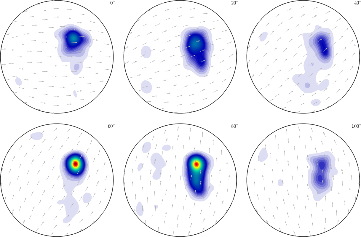
- Note that only the fundamental region with respect to the symmetry is plotted
- you can plot the entire orientation space using the argument
'complete'
In most subclasses of SO3Fun the symmetries are independent from the rest of variables of the function. So one can change them very easy and only effects the function values.
SO3F.SLeft = crystalSymmetry('432')SO3F = SO3FunRBF (Quartz → 432)
multimodal components
kernel: de la Vallee Poussin, halfwidth 5°
center: 19848 orientations, resolution: 5°
weight: 1The class SO3FunHarmonic describes an rotational function by the Fourier coefficients of its harmonic series. Here it is possible to get the symmetries directly from the fourier coefficients.
Similarly, if we want to change the symmetry of a function it is not enough to change it. We also have to symmetries this function.
SO3F2 = SO3FunHarmonic(rand(1e3,1))
SO3F2.isReal = true
SO3F2.fhat(1:10)
SO3F2 = SO3FunHarmonic (y↑→x → y↑→x)
isReal: false
bandwidth: 9
weight: 0.44
SO3F2 = SO3FunHarmonic (y↑→x → y↑→x)
bandwidth: 9
weight: 0.44
ans =
0.4353
0.2775
0.4297
0.4129
0.4430
0.2997
0.4430
0.4129
0.4297
0.2775plot(SO3F2)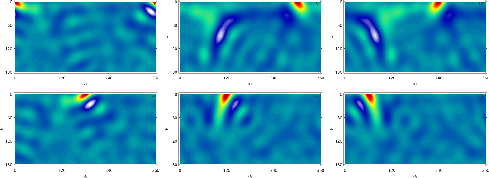
Changing the symmetry has no effect on the Fourier coefficients. Now we are only plotting the given function on some fundamental region.
SO3F2.SRight = crystalSymmetry('2')
SO3F2.fhat(1:10)
SO3F2 = SO3FunHarmonic (121 → y↑→x)
bandwidth: 9
weight: 0.44
ans =
0.4353
0.2775
0.4297
0.4129
0.4430
0.2997
0.4430
0.4129
0.4297
0.2775plot(SO3F2)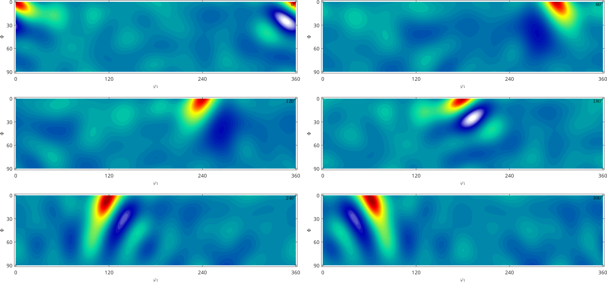
Symmetrising the Fourier coefficients transforms the coefficients. So we symmetrise the function and it is no longer possible to go back to the non symmetrised function from before.
SO3F2 = SO3F2.symmetrise
SO3F2.fhat(1:10)
SO3F2 = SO3FunHarmonic (121 → y↑→x)
bandwidth: 9
weight: 0.44
ans =
0.4353
-0.0677
0
0.0677
0
0
0
0.0677
0
-0.0677plot(SO3F2)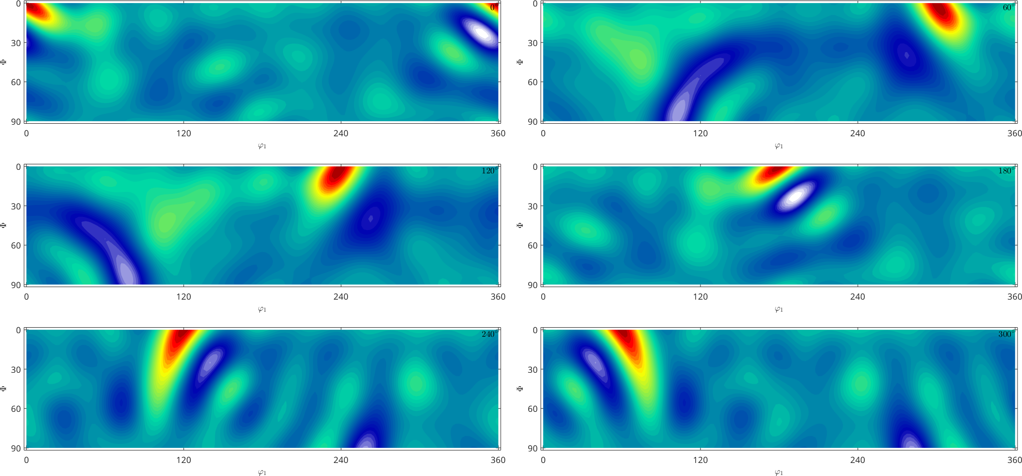
Now the function is symmetrised on the full rotation group.
plot(SO3F2,'complete')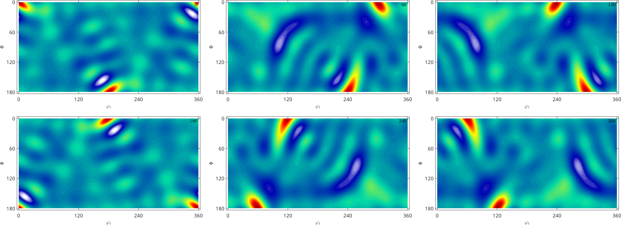
Note that you can expand every SO3Fun to an SO3FunHarmonic
SO3F3 = SO3FunHarmonic(SO3F)SO3F3 = SO3FunHarmonic (Quartz → 432)
bandwidth: 48
weight: 1and do the same as before.