Advanced Grain Reconstruction

Grain Reconstruction introduced the threshold angle, 'alpha', and 'minPixel'. This page shows how to replace parts of the reconstruction rather than tune those three settings.

A grain is a phase-homogeneous, spatially connected region of EBSD pixels produced by segmentation. This page assumes that definition and the basic reconstruction workflow. If misorientation is new to you, first see Misorientation Theory.

It helps to separate calcGrains into three operations:

The first sections replace the second operation. The later sections compare two spatial decompositions used by the first. Denoising orientations and filling missing orientations are separate preprocessing decisions; see Denoising Orientation Maps and Fill Missing Data in Orientation Maps.

We use the same subregion of the forsterite data set as the basic page.

plottingConvention.default('y↑→x');
mtexdata forsterite silent
ebsd = ebsd(inpolygon(ebsd,[5 2 10 5]*10^3));

The grain boundary criterion

A grainBoundaryCriterion evaluates arrays of neighbouring pixel indices at once. It returns one connectivity per pair, from 0 for separated to 1 for fully connected. The discrete angle criterion uses three values:

Without clustering, every positive connectivity joins the graph used to form grains. A connectivity at or below 0.5 is also drawn as a boundary. A continuous criterion can therefore draw a boundary between two cells that remain connected through the grain. The soft-threshold example below makes this distinction visible.

Normally calcGrains constructs a criterion from its options. It also accepts a criterion object directly. These calls perform the same reconstruction, so their summaries would only repeat one another.

[grainsUniform,ebsdUniform] = ...
  calcGrains(ebsd,'angle',10*degree,'minPixel',5);
[grainsFromObject,ebsdFromObject] = ...
  calcGrains(ebsd,gbcAngle(10*degree),'minPixel',5);

fprintf('Option and criterion object give identical grain ids: %d\n',...
  isequal(ebsdUniform.grainId,ebsdFromObject.grainId));

Option and criterion object give identical grain ids: 1

MTEX supplies gbcAngle, gbcSoft, gbcCustom, gbcVariants, and gbcFMC. The default is gbcAngle. The basic page uses gbcFMC for deformed microstructures. The criterion gbcVariants separates variant ids during parent grain reconstruction. The three remaining alternatives are developed here.

Phase-dependent thresholds

Different phases may require different boundary angles. A cell array gives one threshold per phase, in the order of ebsd.CSList. Its displayed summary makes that order explicit.

ebsd.CSList

ans = 
    mineral         color  symmetry        a, b, c    reference frame
 notIndexed          none                                            
 Forsterite  LightSkyBlue       mmm     4.8, 10, 6                   
  Enstatite  DarkSeaGreen       mmm   18, 8.8, 5.2                   
   Diopside     Goldenrod     12/m1    9.7, 9, 5.3  X||a*, Y||b, Z||c
    Silicon    LightCoral      m-3m  5.4, 5.4, 5.4

The first entry is notIndexed. It is never used as an angular threshold, but it must be present. The other four entries belong to the four minerals. Here forsterite, the phase that carries the deformation in this specimen, is separated at 5 degrees. The other phases keep the 10 degree threshold.

threshold = {10*degree, ...  % notIndexed, never used
  5*degree, ...              % Forsterite
  10*degree, ...             % Enstatite
  10*degree, ...             % Diopside
  10*degree};                % Silicon

grainsPhase = calcGrains(ebsd,'angle',threshold,'minPixel',5);

fprintf('Forsterite grains: uniform 10 degree = %d; phase-dependent = %d\n',...
  length(grainsUniform('Forsterite')),length(grainsPhase('Forsterite')));

Forsterite grains: uniform 10 degree = 55; phase-dependent = 63

The printed counts show that the lower forsterite threshold splits that phase more finely. The other phases use exactly the same criterion as in the uniform reconstruction and are unchanged.

An entry may itself be a pair [highAngle lowAngle]. The first angle separates grains; the second records internal boundaries. See Subgrain Boundaries for that distinction.

Soft thresholds

A hard threshold is discontinuous in the data. Neighbouring pixels 9.9 degrees apart remain together, while pixels 10.1 degrees apart separate, although the physical distinction is unlikely to be that sharp.

gbcSoft replaces the step with an error function. Its two parameters are the centre angle and transition width. Connectivity then decreases gradually across the band.

grainsSoft = calcGrains(ebsd,gbcSoft([10 2]*degree),'minPixel',5);
grainsHard14 = calcGrains(ebsd,'angle',14*degree,'minPixel',5);

softPhaseCounts = accumarray(grainsSoft.phaseId,1,...
  [length(ebsd.CSList),1]);
hardPhaseCounts = accumarray(grainsHard14.phaseId,1,...
  [length(ebsd.CSList),1]);

fprintf('Soft [10 2] and hard 14 degree phase counts agree: %d\n',...
  isequal(softPhaseCounts,hardPhaseCounts));
fprintf('Soft-criterion boundary segments inside grains: %d\n',...
  length(grainsSoft.innerBoundary));

Soft [10 2] and hard 14 degree phase counts agree: 1
Soft-criterion boundary segments inside grains: 28

On its own, the soft criterion still forms grains from positive graph connections. The error function reaches numerical zero only after its transition has saturated, so this example merely raises the effective splitting angle. Its phase counts match a hard 14 degree threshold.

The fractional values still record the transition band. A pair past the centre can have a boundary drawn while remaining connected inside its grain. Those weights become useful when Markovian Clustering replaces connected components with a weighted graph clustering.

Segmenting by another per-pixel property

gbcCustom separates neighbouring pixels when a supplied per-pixel property differs by more than a threshold. The property may be numeric, a vector3d, or a quaternion. Vectors and quaternions are compared by their angle.

The custom criterion compares only that property; it does not add a phase check. Subset a multiphase map to one phase, as below, or enforce phase separation in a criterion of your own. This keeps the resulting grains phase-homogeneous.

Here grains are defined by their c-axis alone. Two forsterite pixels may belong to the same grain whenever their c-axes agree, regardless of the rotation about that axis.

fo = ebsd('Forsterite');
cAxis = fo.orientations .* Miller(0,0,1,fo.CS);

grainsC = calcGrains(fo,...
  gbcCustom(cAxis,10*degree,'antipodal'),'minPixel',5);
grainsA = calcGrains(fo,'angle',10*degree,'minPixel',5);

fprintf('Full-orientation grains: %d; c-axis grains: %d\n',...
  length(grainsA),length(grainsC));

Full-orientation grains: 69; c-axis grains: 66

The flag 'antipodal' is passed to angle. It makes the c-axis an axis rather than a direction. Without it, opposite senses of the same axis would be treated as different.

Draw the ordinary reconstruction in black and the c-axis reconstruction in red. Black segments that remain visible mark boundaries across which the c-axes agree but the rotations about them differ.

ipfKey = ipfColorKey(fo.CS);
ipfColor = ipfKey.orientation2color(fo.orientations);

plot(fo,ipfColor,'micronbar','off')
hold on
plot(grainsA.boundary,'linewidth',3,'lineColor','black')
plot(grainsC.boundary,'linewidth',1,'lineColor','red')
hold off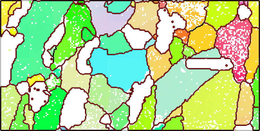

Only a few black segments remain on this specimen. The printed counts show that 69 full-orientation grains become 66 c-axis grains. Such mergers would be more common in a material with a strong fibre texture.

Writing your own criterion

A custom criterion is a subclass of grainBoundaryCriterion. Implement the protected method doEvaluate(obj,ebsd,i,j). The arrays i and j list neighbouring pixel indices and the output must have the same size.

This example requires both a small misorientation and adequate band contrast. The second condition stops a grain from leaking through a chain of poorly indexed pixels. The value minBC = 50 is specific to the data and acquisition settings; inspect the band-contrast distribution before choosing it.

classdef gbcAngleAndBC < grainBoundaryCriterion

properties
  threshold = 10*degree
  minBC = 50
end

methods (Access = protected)

   function out = doEvaluate(obj,ebsd,i,j)

     % delegate the misorientation part
     out = eval(gbcAngle(obj.threshold),ebsd,i,j);

     % veto connections through low band contrast
     bad = ebsd.bc(i) < obj.minBC | ebsd.bc(j) < obj.minBC;
     out(bad) = 0;

   end
 end
 end

Save the class as gbcAngleAndBC.m on the MATLAB search path. It can then be passed like any other criterion:

grains = calcGrains(ebsd,gbcAngleAndBC,'minPixel',5)

The base class also defines prepare(obj,ebsd) for subclasses that need information from the whole map. At present, calcGrains does not call this hook automatically. Precompute that information before constructing the criterion, or call an overloaded prepare explicitly.

The spatial decomposition

The option 'alpha' changes the first reconstruction operation: the spatial support from which cells are built. By default, MTEX closes the indexed region with a raster disk whose radius is alpha pixel spacings. A notIndexed region narrower than 2*alpha is crossed by surrounding cells; a wider region remains a separate notIndexed grain. The default is alpha = 3.1.

The work of raster closing grows with the area of the disk. The flag 'delaunay' instead computes a Delaunay triangulation of the indexed pixels. A triangle is included when its circumradius is at most alpha pixel spacings. This is an exact alpha complex rather than a raster approximation, and its cost changes little as 'alpha' grows. Raster closing is faster near the default; the Delaunay route is intended for maps with gaps wide enough to require a large value.

tic
grainsRaster = calcGrains(ebsd,'angle',10*degree,...
  'minPixel',5,'alpha',60);
toc

tic
grainsDelaunay = calcGrains(ebsd,'angle',10*degree,...
  'minPixel',5,'alpha',60,'delaunay');
toc

Elapsed time is 5.029164 seconds.
Elapsed time is 3.292552 seconds.

The elapsed times are machine-dependent; their contrast is the result to notice. The two decompositions also need not agree pixel for pixel at the same value because closing radius and circumradius are different geometric quantities.

Diagnose the notIndexed regions first

Choosing one 'alpha' for a whole map need not be guesswork. calcGrains returns connected notIndexed areas as grains, so their size and shape can be inspected with the tools from Shape Parameters. Setting alpha = 0 closes nothing, so narrow notIndexed areas stay where they are instead of being absorbed into their neighbours.

[grainsOpen,ebsdOpen] = calcGrains(ebsd,'angle',10*degree,'alpha',0);
notIndexedGrains = grainsOpen('notIndexed')

notIndexedGrains = grain2d (y↑→x)
 
 Phase  Grains  Pixels     Mineral  Symmetry  Color
     0    1064    3229  notIndexed             none
 
 boundary segments: 7456 (372800 µm)
 inner boundary segments: 0 (0 µm)
 triple points: 807
 
 Properties: meanRotation, GOS

Pixel counts give a first scale estimate. The equivalent-circle radius of a region with n pixels is sqrt(n/pi) pixel spacings.

numPixel = notIndexedGrains.numPixel;
sizeSummary = table(median(numPixel),quantile(numPixel,0.99),...
  max(numPixel),sqrt(max(numPixel)/pi),...
  'VariableNames',{'medianPixels','p99Pixels','maxPixels',...
  'maxEquivalentRadiusPixels'})

sizeSummary =
  1×4 table
    medianPixels    p99Pixels    maxPixels    maxEquivalentRadiusPixels
    ____________    _________    _________    _________________________
         1             30           355                 10.63

The table shows that most areas are isolated failed measurements, while a few are regions in their own right. The largest contains 355 pixels and has an equivalent-circle radius of about 10.6 pixels. This radius suggests the scale to inspect; it does not predict the closing value by itself. Closing responds to the narrowest width and therefore also to shape.

The ratio below is a quick size-and-compactness diagnostic. It is high for large, compact blobs and low for small or ragged areas. It is not a scale-free compactness measure because the numerator grows with area and the denominator counts boundary segments. Use shapeFactor when shape must be compared apart from size.

plot(notIndexedGrains,...
  log(notIndexedGrains.numPixel ./ notIndexedGrains.boundarySize))
mtexColorbar('title','log(pixels / boundary segments)')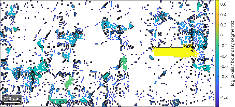

High colours identify the larger, more compact holes that can justify preservation. Low colours mark isolated pixels and ragged indexing failures that a closing may reasonably absorb. The map is a diagnostic, not an automatic choice of 'alpha'.

A notIndexed pixel and an absent grid position have different experimental meanings. The first is a real measurement whose pattern could not be indexed; the second has no retained measurement. The spatial decomposition treats both as positions without an indexed orientation, so 'alpha' acts on both. Deleting measurements therefore creates a gap for segmentation; it does not assign orientations there. To reconstruct orientations, see Fill Missing Data in Orientation Maps.

Choosing the next step

Use a custom criterion when the physical separator is another per-pixel quantity. Use the spatial options when the uncertainty is where the map has support. In either case, repeat the reconstruction over defensible nearby settings before treating a grain count or size distribution as measured.

Continue with Markovian Clustering when fractional criterion weights should influence the grouping itself. The resulting boundaries and their internal boundaries are developed in Grain Boundaries and Subgrain Boundaries. Standards for reporting EBSD grain size are listed on the basic reconstruction page.

References

- F. Bachmann, R. Hielscher, and H. Schaeben, Grain Detection from 2d and 3d EBSD Data---Specification of the MTEX Algorithm, Ultramicroscopy 111 (2011), 1720--1733. This paper derives the Voronoi reconstruction used by
calcGrains. - H. Edelsbrunner, D. G. Kirkpatrick, and R. Seidel, On the Shape of a Set of Points in the Plane, IEEE Transactions on Information Theory 29 (1983), 551--559. This paper introduces planar alpha shapes.
- P. Soille, Morphological Image Analysis: Principles and Applications, 2nd ed., Springer, 2003. The chapters on dilation, erosion, opening, and closing provide the image-processing basis for the raster decomposition.
Citing this page.
This page is part of the documentation of
MTEX, a free and open
source MATLAB toolbox for analyzing and modeling crystallographic textures.
It was written by The MTEX Developers and is published at
https://mtex-toolbox.github.io/GrainReconstructionAdvanced.html.
If you use MTEX, or reuse text or figures from this page, in your research,
please cite
F. Bachmann, R. Hielscher, H. Schaeben: Texture Analysis with MTEX - Free and Open Source Software Toolbox, Solid State Phenomena 160 (2010), 63-68. 10.4028/www.scientific.net/SSP.160.63
BibTeX
@article{bachmann2010mtex,
author  = {F. Bachmann and R. Hielscher and H. Schaeben},
title   = {Texture Analysis with MTEX - Free and Open Source Software Toolbox},
journal = {Solid State Phenomena},
volume  = {160},
pages   = {63-68},
year    = {2010},
doi     = {10.4028/www.scientific.net/SSP.160.63},
url     = {https://doi.org/10.4028/www.scientific.net/SSP.160.63}
}
Other papers describing specific MTEX methods are listed under Publications — please cite the one that best fits your application. The MTEX source code is licensed under the GNU General Public License v2.0; the text and figures of this documentation are licensed under CC BY 4.0, which permits reuse — including by automated systems — provided The MTEX Developers and this page are credited.