Crystal Orientation as Coordinate Transformation

An orientation in MTEX maps crystal coordinates to specimen coordinates. It takes a direction or tensor expressed in the crystal frame and returns the same object expressed in the specimen frame.

A reference frame is the coordinate system in which data are expressed. The crystal frame is the Cartesian frame fixed to a phase's lattice, while the specimen frame describes the sample in a measurement, rolling, or geological frame.

This page assumes the Miller indices introduced in Crystal Directions and the active rotations from Rotation Operations. Everything below follows from the direction of the coordinate map, including which side a rotation acts on and what happens when the specimen is turned.

plottingConvention.default('y↑→x');

The Two Ingredients

An orientation combines a rotation with the symmetry, lattice metric, and crystal frame stored by a crystalSymmetry.

rot = rotation.byEuler(10*degree,20*degree,30*degree,'Bunge');

cs = crystalSymmetry.load("Al-Aluminum.cif")

cs = crystalSymmetry (⊙c→a)
 
  mineral : Aluminum
  symmetry: m3̅m    
  elements: 48      
  a, b, c : 4, 4, 4

The summary identifies aluminium, its point group, lattice parameters, and crystal-frame alignment. Combining rot and cs gives an orientation.

ori = orientation(rot,cs)

ori = orientation (Aluminum → y↑→x)
 
  Bunge Euler angles in degree
  phi1  Phi phi2
    10   20   30

The arrow in the summary reads from the crystal frame on the left to the specimen frame on the right. An orientation is also a rotation, so every rotation operation applies to it.

From Crystal Coordinates to Specimen Coordinates

Take the crystal direction \([100]\).

h = Miller(1,0,0,cs,'uvw');

In a grain with orientation ori, that direction has the following Cartesian components in the specimen frame.

r = ori * h

r = vector3d (y↑→x)
     x     y     z
  3.12  2.48 0.693

The picture shows the same map. The translucent cube is the crystal where ori places it. The black arrows are the specimen axes X, Y and Z, and the red arrow is the crystal direction h expressed in specimen coordinates. The direction is fixed in the lattice; what the orientation supplies is where the lattice is pointing.

cS = crystalShape.cube(cs);

figure;
plot(ori * cS,'faceAlpha',0.35,'faceColor',[0.6 0.75 0.9]);
hold on;
arrow3d(0.75*normalize(r),'faceColor','red');
arrow3d(0.75*[vector3d.X,vector3d.Y,vector3d.Z],...
  'faceColor','black');
hold off;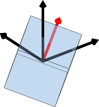

Other Crystal Objects Transform the Same Way

The same multiplication applies to a stiffness tensor. This example starts with tensor components in the crystal frame.

C = stiffnessTensor(...
  [[2 1 1 0 0 0];...
  [1 2 1 0 0 0];...
  [1 1 2 0 0 0];...
  [0 0 0 1 0 0];...
  [0 0 0 0 1 0];...
  [0 0 0 0 0 1]],cs)

C = stiffnessTensor (Aluminum)
  unit: GPa              
  rank: 4 (3 × 3 × 3 × 3)
 
  tensor in Voigt matrix representation:
 2 1 1 0 0 0
 1 2 1 0 0 0
 1 1 2 0 0 0
 0 0 0 1 0 0
 0 0 0 0 1 0
 0 0 0 0 0 1

After the coordinate transform, the summary names the specimen frame and displays the transformed components.

Cspecimen = ori * C

Cspecimen = stiffnessTensor (y↑→x)
  unit: GPa              
  rank: 4 (3 × 3 × 3 × 3)
 
  tensor in Voigt matrix representation:
  2.4848  0.5709  0.9443 -0.1463 -0.0033 -0.0994
  0.5709  2.5851   0.844 -0.1116  0.0399  0.0558
  0.9443   0.844  2.2117  0.2579 -0.0367  0.0436
 -0.1463 -0.1116  0.2579   0.844  0.0436  0.0399
 -0.0033  0.0399 -0.0367  0.0436  0.9443 -0.1463
 -0.0994  0.0558  0.0436  0.0399 -0.1463  0.5709

Everything defined in the crystal frame travels in the same direction:

And Back Again

The inverse orientation maps specimen coordinates to crystal coordinates. Applying it to r therefore returns the direction we started from.

hBack = inv(ori) * r

hBack = Miller (Aluminum)
        h       k       l
  16.3991       0       0

The displayed coefficients do not resemble \([100]\) yet. A Miller made from a specimen direction displays as \((hkl)\) unless told otherwise, while the original \([100]\) direction has the aluminium lattice-vector length of 4.04958 Angstrom. Selecting lattice-direction notation and rounding recovers the original indices.

hBack.dispStyle = 'uvw';
hRounded = round(hBack)

hRounded = Miller (Aluminum)
  u v w
  1 0 0

Much of the literature defines an orientation in the opposite direction, from specimen to crystal coordinates. That is what MTEX calls inv(ori). Both conventions are in use, and reading Euler angles with the wrong one inverts every orientation in the data. See MTEX vs. Bunge Convention for the practical consequences.

Turning the Specimen

Putting the sample on the stage in another position actively turns the crystal relative to the fixed measurement frame. A rotation expressed in specimen coordinates therefore multiplies every orientation from the left.

rotSpecimen = rotation.byAxisAngle(vector3d.X,60*degree);
oriNew = rotSpecimen * ori;

Every crystal direction moves with the specimen. Going through the new orientation and turning the old specimen direction must agree.

leftConsistency = angle(oriNew * h,rotSpecimen * r) ./ degree

leftConsistency =
   1.2074e-06

The residual is numerically zero. The same rotation written on the right is interpreted in crystal coordinates: it turns the direction inside the lattice before ori maps that direction into the specimen frame.

rightDifference = angle(ori * (rotSpecimen * h),oriNew * h) ./ degree

rightDifference =
   37.1140

The nonzero result confirms that left and right multiplication describe different operations. The rotation on the right acts first, just as in ordinary matrix multiplication.

Crystal Symmetry Also Acts from the Right

Right multiplication has a second, symmetry-aware meaning. A point-group operation changes the crystal-frame representative but not the physical crystal setting. symmetrise lists those equivalent descriptions.

equivalentCounts = [length(ori.symmetrise),...
  length(ori.symmetrise('proper'))]

equivalentCounts =
    48    24

The first count is 48, the number of elements in aluminium's m-3m point group. The second count is 24, because only the proper operations are rigid rotations. The 24 improper operations remain symmetries of the lattice and are relevant when opposite plane normals are treated as equivalent.

A symmetry-aware orientation comparison regards all 48 descriptions as equivalent. Their largest angular difference from ori is only a floating-point residual.

symmetryResidual = max(angle(ori.symmetrise,ori)) ./ degree

symmetryResidual =
   3.4151e-06

Rotating Is Not Changing Frame

The stage rotation above moves the physical object in a fixed frame. A frame change instead re-expresses the same physical object in another reference frame and leaves the object untouched. Use transformReferenceFrame when crystal data use a different Cartesian crystal frame. Orientations also depend on how the Cartesian crystal frame \(\vec x\), \(\vec y\), \(\vec z\) is inscribed into the crystal axes \(\vec a\), \(\vec b\), \(\vec c\).

A plotting convention only states how a reference frame is laid out on screen. Changing it does not rotate the specimen or re-express the data. The Crystal Reference System develops both distinctions for crystal axes.

The Maths Behind the Multiplication Order

Let \(\mathbf{G}\) be the matrix of ori, and let \(\mathbf{h}\) and \(\mathbf{r}\) contain the crystal and specimen components of one direction. Then

\[ \mathbf{r} = \mathbf{G}\mathbf{h}, \qquad \mathbf{h} = \mathbf{G}^{\mathrm{T}}\mathbf{r}. \]

The transpose appears because a rotation matrix is orthogonal, so \(\mathbf{G}^{-1}=\mathbf{G}^{\mathrm{T}}\). A specimen rotation \(\mathbf{Q}\) gives \(\mathbf{QG}\), while a crystal-frame rotation \(\mathbf{P}\) gives \(\mathbf{GP}\). This is the matrix form of the two multiplication examples above.

The same rule determines the order of a misorientation product. See Misorientations.

References

Next

Symmetry develops the equivalent rotations that an orientation represents. Pole Figures then draws the specimen directions computed here, while Inverse Pole Figures asks the inverse question.

References

- H.-J. Bunge, Texture Analysis in Materials Science: Mathematical Methods, Butterworths, English ed., 1982, establishes the Euler-angle and orientation conventions used in texture analysis.
- A. Morawiec, Orientations and Rotations: Computations in Crystallographic Textures, Springer, 2004, develops coordinate maps, symmetry, and the geometry of orientation space.
- D. Rowenhorst et al., Consistent representations of and conversions between 3D rotations, Modelling and Simulation in Materials Science and Engineering 23, 083501, 2015, compares active and passive conventions and gives reproducible conversion rules.
- ISO 24173:2024, Microbeam analysis -- Guidelines for orientation measurement using electron backscatter diffraction, gives current guidance for reproducible EBSD orientation measurements.