The Schmid factor \(\tau\) is a purely geometric quantity that describes how well a slip system is aligned to a specific tension direction or stress tensor. A Schmid factor \(\tau=0\) indicates that the slip system can not be active since either the tension direction is perpendicular to the slip direction or the normal direction of the slip plane.
In order to investigate this quantity in more detail lets consider an fcc material with its dominant \([0 1 \bar{1}](1 1 1)\) slip system and tension in direction \(r = (001)\)
% define symmetry and slip system
cs = crystalSymmetry('cubic',[3.523,3.523,3.523],'mineral','Nickel');
sS = slipSystem.fcc(cs)

r = vector3d.Z;
sS = slipSystem (Nickel)
u v w | h k l CRSS
0 1 -1 1 1 1 1Lets visualize the situation
% define and plot the crystal shape
cS = crystalShape.cube(cs);
plot(cS,'faceAlpha',0.5)
hold on
plot(cS,sS,'facecolor','blue','label','b')
arrow3d(-0.8*sS.n,'faceColor','black','linewidth',2,'label','n')
plottingConvention.default3D().setView

arrow3d(0.4*r,'faceColor','red','linewidth',2,'label','r')
hold off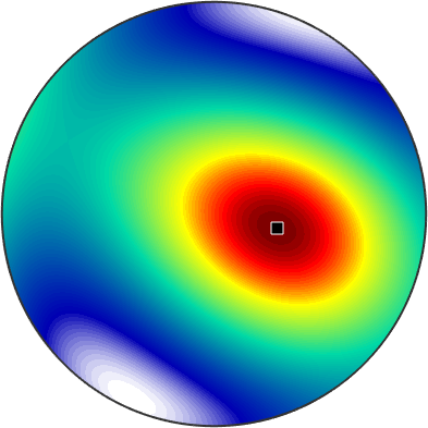
Definition of the Schmid factor
The Schmid factor \(\tau\) is defined as the product of the cosines of the angles between the tension direction \(\vec r\) with the normal direction \(\vec n=(1 1 1)\) and the Burgers vector \(\vec b=[0 1 \bar{1}]\) of the slip system:
\[\tau = \cos \angle(\vec r,\vec n) \cdot \cos \angle(\vec r,\vec b) \]
tau = cos(angle(r,sS.n,'noSymmetry')) * cos(angle(r,sS.b,'noSymmetry'))tau =
-0.4082The same computation can be performed more comfortably using the command SchmidFactor
sS.SchmidFactor(r)ans =
-0.4082Omitting the tension direction r the command SchmidFactor returns the Schmid factor as a spherical function of type S2FunHarmonic which can be used for visualization or detecting the tension directions with highest / lowest Schmid factor.
SF = sS.SchmidFactor
% plot the Schmid factor in dependency of the tension direction
plot(SF)
% find the tension directions with the maximum Schmid factor
[SFMax,pos] = max(SF)
% and annotate them
annotate(pos)SF = S2FunHarmonic (Nickel)
bandwidth: 4
antipodal: true
SFMax =
0.5000
pos = Miller (Nickel)
antipodal: true
h k l
-1.4387 -3.1996 0.3231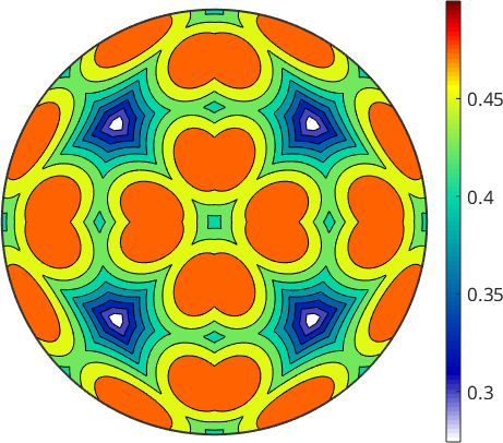
The Schmid factor for general stress tensors
Instead by the tension direction r the stress might be specified by a stressTensor sigma
sigma = stressTensor.uniaxial(r)sigma = stressTensor (y↑→x)
rank: 2 (3 x 3)
0 0 0
0 0 0
0 0 1Then the Schmid factor for the slip system sS and the stress tensor sigma is computed by
sS.SchmidFactor(sigma)Warning: The reference system of the stress tensor and the slip systems do not
match!
ans =
-0.4082Multiple Slip Systems
In general a crystal contains not only one slip system but at least all symmetrically equivalent ones. Those can be computed with
sSAll = sS.symmetrise('antipodal')sSAll = slipSystem (Nickel)
size: 12 x 1
u v w | h k l CRSS
0 1 -1 1 1 1 1
-1 0 1 1 1 1 1
1 -1 0 1 1 1 1
1 -1 0 1 1 -1 1
1 0 1 1 1 -1 1
0 1 1 1 1 -1 1
0 1 -1 -1 1 1 1
1 0 1 -1 1 1 1
1 1 0 -1 1 1 1
-1 0 1 1 -1 1 1
1 1 0 1 -1 1 1
0 1 1 1 -1 1 1The option 'antipodal' indicates that Burgers vectors in opposite direction should not be distinguished. Lets visualize the situation
close all
t = tiledlayout(3,4,'TileSpacing','tight','Padding','tight', 'TileIndexing', 'columnmajor');
for k = 1:length(sSAll)
  ax = nexttile;
  plot(cS,'faceAlpha',0.5,'parent',ax)
  title(ax,['\textbf{' int2str(k) '}:' char(sSAll(k),'latex')],'Interpreter','latex')
  axis off
  hold on
  plot(cS,sSAll(k),'facecolor','blue','parent',ax)
  plottingConvention.default3D().setView
  arrow3d(0.4*r,'faceColor','red','linewidth',3)
  hold off
end
Computing the Schmid factors for all those slip systems simultaneously by
tau = sSAll.SchmidFactor(r)tau =
Columns 1 through 7
-0.4082 0.4082 0.0000 -0.0000 -0.4082 -0.4082 -0.4082
Columns 8 through 12
0.4082 0.0000 0.4082 0.0000 0.4082returns a list of Schmid factors and we can find the slip system with the largest Schmid factor using
[tauMax,id] = max(abs(tau))

sSAll(id)
tauMax =
0.4082
id =
12
ans = slipSystem (Nickel)
u v w | h k l CRSS
0 1 1 1 -1 1 1The above computation can be easily extended to a list of tension directions. This allows us to display the maximum Schmid factor over all slip systems as a function of the tension direction.
% define a grid of tension directions
r = plotS2Grid('resolution',0.5*degree,'upper');

% compute the Schmid factors for all slip systems and all tension
% directions
tau = sSAll.SchmidFactor(r);

% tau is a matrix with columns representing the Schmid factors for the
% different slip systems. Lets take the maximum row-wise
[tauMax,id] = max(abs(tau),[],2);

% visualize the maximum Schmid factor as a function of the tension
% direction
contourf(r,tauMax)
mtexColorbar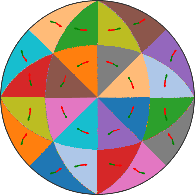
We may also plot the index of the active slip system as a function of the tension direction
pcolor(r,id)

mtexColorMap(vega20(12))
and observe that within the fundamental sectors the active slip system remains the same. Lets annotate which are the active slip systems
% take as directions the centers of the fundamental regions
rCenter = symmetrise(cs.fundamentalSector.center,cs);
rCenter = rCenter(rCenter.z>=0);

% compute the Schmid factor
tau = sSAll.SchmidFactor(rCenter);

% find the slip system with the maximum Schmid factor
[~,id] = max(abs(tau),[],2);

% display the slip system with the maximum Schmid factor
hold on
for k = 1:length(rCenter)
 text(rCenter(k),char(sSAll(id(k)),'latex'),'Interpreter','latex')
end
hold off
If we perform this computation in terms of spherical functions we obtain
% omitting |r| gives us a list of 12 spherical functions
tau = sSAll.SchmidFactor

% now we take the max of the absolute value over all these functions
contourf(max(abs(tau),[],1),'upper')
mtexColorbar
tau = S2FunHarmonic (Nickel)
size: 12 x 1
bandwidth: 4
antipodal: true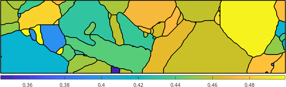
The Schmid factor for EBSD data
So far we have always assumed that the stress tensor is already given relatively to the crystal coordinate system. Next, we want to examine the case where the stress is given in specimen coordinates and we know the orientation of the crystal. Let's import some EBSD data and compute the grains
mtexdata csl

% take some subset
ebsd = ebsd(ebsd.inpolygon([0,0,200,50]))

grains = calcGrains(ebsd);
grains = smooth(grains,5);

plot(ebsd,ebsd.orientations,'micronbar','off')
hold on
plot(grains.boundary,'linewidth',2)
hold off
ebsd = EBSD (y↑→x)
Phase Orientations Mineral Color Symmetry Crystal reference frame
0 5 (0.0032%) notIndexed
-1 154107 (100%) iron LightSkyBlue m-3m
Properties: ci, error, iq
Scan unit : um
X x Y x Z : [0, 511] x [0, 300] x [0, 0]
Normal vector: (0,0,1)
ebsd = EBSD (y↑→x)
Phase Orientations Mineral Color Symmetry Crystal reference frame
-1 10251 (100%) iron LightSkyBlue m-3m
Properties: ci, error, iq
Scan unit : um
X x Y x Z : [0, 200] x [0, 50] x [0, 0]
Normal vector: (0,0,1)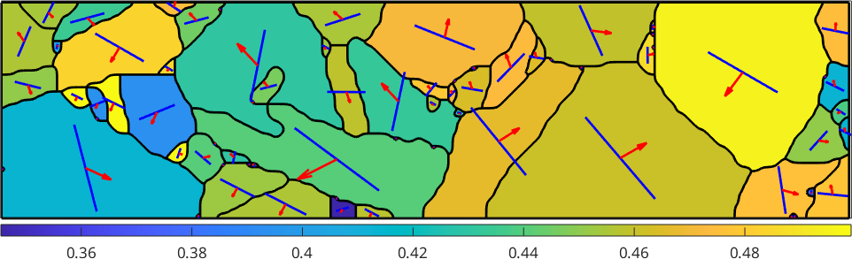
We want to consider the following slip systems
sS = slipSystem.fcc(ebsd.CS)
sS = sS.symmetrise;
sS = slipSystem (iron)
u v w | h k l CRSS
0 1 -1 1 1 1 1Since, those slip systems are in crystal coordinates but the stress tensor is in specimen coordinates we either have to rotate the slip systems into specimen coordinates or the stress tensor into crystal coordinates. In the following sections we will demonstrate both ways. Lets start with the first one
% rotate slip systems into specimen coordinates
sSLocal = grains.meanOrientation * sS
sSLocal = slipSystem (y↑→x)
CRSS: 1
size: 71 x 24These slip systems are now arranged in matrix form where the rows correspond to the crystal reference frames of the different grains and the columns are the symmetrically equivalent slip systems. Computing the Schmid factor we end up with a matrix of the same size
% compute Schmid factor
sigma = stressTensor.uniaxial(vector3d.Z)
SF = sSLocal.SchmidFactor(sigma);

% take the maximum along the rows
[SFMax,active] = max(SF,[],2);

% plot the maximum Schmid factor
plot(grains,SFMax,'micronbar','off','linewidth',2)
mtexColorbar location southoutside
sigma = stressTensor (y↑→x)
rank: 2 (3 x 3)
0 0 0
0 0 0
0 0 1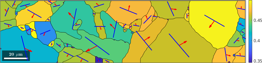
Next we want to visualize the active slip systems.
% take the active slip system and rotate it in specimen coordinates
sSactive = grains.meanOrientation .* sS(active);

hold on
% visualize the trace of the slip plane
quiver(grains,sSactive.trace,'color','b')

% and the slip direction
quiver(grains,sSactive.b,'color','r')
hold off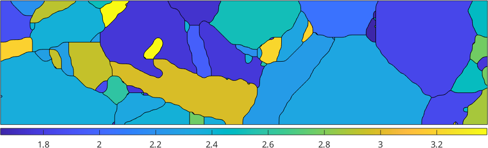
We observe that the Burgers vector is in most case aligned with the trace. In those cases where trace and Burgers vector are not aligned the slip plane is not perpendicular to the surface and the Burgers vector sticks out of the surface.
Next we want to demonstrate the alternative route
% rotate the stress tensor into crystal coordinates
sigmaLocal = inv(grains.meanOrientation) * sigma
sigmaLocal = stressTensor (iron)
size: 71 x 1
rank: 2 (3 x 3)This becomes a list of stress tensors with respect to crystal coordinates - one for each grain. Now we have both the slip systems as well as the stress tensor in crystal coordinates and can compute the Schmid factor
% the resulting matrix is the same as above
SF = sS.SchmidFactor(sigmaLocal);

% and hence we may proceed analogously
% take the maximum along the rows
[SFMax,active] = max(SF,[],2);

% plot the maximum Schmid factor
plot(grains,SFMax)
mtexColorbar

% take the active slip system and rotate it in specimen coordinates
sSactive = grains.meanOrientation .* sS(active);

hold on
% visualize the trace of the slip plane
quiver(grains,sSactive.trace,'color','b')

% and the slip direction
quiver(grains,sSactive.b,'color','r')

hold off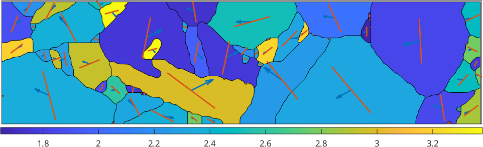
Strain-based analysis on the same data set
eps = strainTensor(diag([1,0,-1]))

epsCrystal = inv(grains.meanOrientation) * eps

[M, b] = calcTaylor(epsCrystal, sS);

plot(grains,M,'micronbar','off')
mtexColorbar southoutside
eps = strainTensor (y↑→x)
type: Lagrange
rank: 2 (3 x 3)
1 0 0
0 0 0
0 0 -1
epsCrystal = strainTensor (iron)
size: 71 x 1
type: Lagrange
rank: 2 (3 x 3)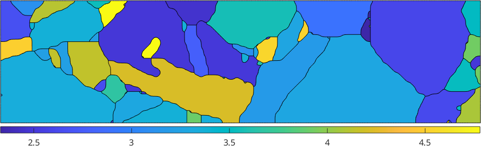
[ bMax , bMaxId ] = max( b , [ ] , 2 ) ;
sSGrains = grains.meanOrientation .* sS(bMaxId) ;
hold on
bVec = sSGrains.b; bVec.z = 0;
quiver ( grains , bVec)
quiver ( grains , sSGrains.trace)
hold off