
A legend pairs a plotted symbol or line with a label. Use one when a small number of discrete objects must be distinguished, such as selected grains, boundary classes, or reference directions.
In MTEX, legend entries are opt in. An object appears only when it is plotted with a 'DisplayName'. This is the opposite of MATLAB's default behaviour. It prevents markers, construction lines, and a colour-coded background from each acquiring an unhelpful entry.
Choose the legend entries
Name only the objects that the reader needs to distinguish. This example names a point and a great circle. The pole at the centre remains unnamed.
plot(vector3d.X,'upper','DisplayName','point')
hold on

circle(vector3d.X,'DisplayName','great circle',...
  'lineColor','r','lineWidth',2)

plot(vector3d.Z,'Marker','p','MarkerSize',30)
hold off

lgd = legend('show');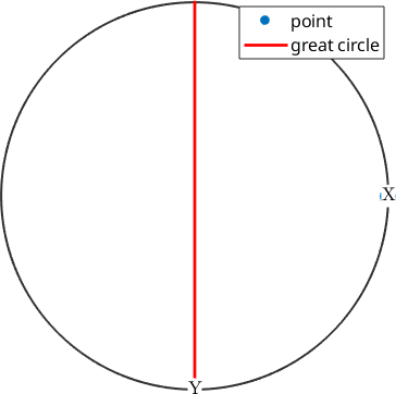
Read and adjust the result
The figure contains three plotted objects, but the legend has two entries. The central star is visible in the axes but absent from the legend because it has no 'DisplayName'.
After MTEX has selected the entries, legend is the ordinary MATLAB legend command. Its returned handle controls the box and its text. For example, an outside location avoids covering the spherical plot, and a title explains what the entries classify.
lgd.Location = 'eastoutside';
lgd.Title.String = 'Geometry';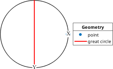
Choose the right colour guide
A legend represents discrete identities. When colour represents a numerical value, use a colour bar because it shows the complete value-to-colour scale. When colour represents a direction or an orientation, use a colour key that maps each possible direction or orientation to a colour. The next page introduces numerical colour scales; IPF Maps explains direction colour keys for orientation maps.
The MATLAB Legend properties provide further controls for placement and styling.
References
- S. R. Midway, Principles of Effective Data Visualization, Patterns 1 (2020), 100141, explains how selective legends and consistent visual scales make plots easier to compare.
Next
Continue with Color Maps to control how numerical values are translated into colours.
Citing this page.
This page is part of the documentation of
MTEX, a free and open
source MATLAB toolbox for analyzing and modeling crystallographic textures.
It was written by The MTEX Developers and is published at
https://mtex-toolbox.github.io/Legends.html.
If you use MTEX, or reuse text or figures from this page, in your research,
please cite
F. Bachmann, R. Hielscher, H. Schaeben: Texture Analysis with MTEX - Free and Open Source Software Toolbox, Solid State Phenomena 160 (2010), 63-68. 10.4028/www.scientific.net/SSP.160.63
BibTeX
@article{bachmann2010mtex,
  author  = {F. Bachmann and R. Hielscher and H. Schaeben},
  title   = {Texture Analysis with MTEX - Free and Open Source Software Toolbox},
  journal = {Solid State Phenomena},
  volume  = {160},
  pages   = {63-68},
  year    = {2010},
  doi     = {10.4028/www.scientific.net/SSP.160.63},
  url     = {https://doi.org/10.4028/www.scientific.net/SSP.160.63}
}
Other papers describing specific MTEX methods are listed under Publications — please cite the one that best fits your application. The MTEX source code is licensed under the GNU General Public License v2.0; the text and figures of this documentation are licensed under CC BY 4.0, which permits reuse — including by automated systems — provided The MTEX Developers and this page are credited.