In this section we consider the analysis of CSL boundaries. Therefore lets start by importing some Iron data and reconstructing the grain structure.
mtexdata csl

% grain segmentation
[grains,ebsd.grainId] = calcGrains(ebsd('indexed'));

% grain smoothing
grains = smooth(grains,5);

% plot the result
plot(grains,grains.meanOrientation)
ebsd = EBSD (y↑→x)
Phase Orientations Mineral Color Symmetry Crystal reference frame
0 5 (0.0032%) notIndexed
-1 154107 (100%) iron LightSkyBlue m-3m
Properties: ci, error, iq
Scan unit : um
X x Y x Z : [0, 511] x [0, 300] x [0, 0]
Normal vector: (0,0,1)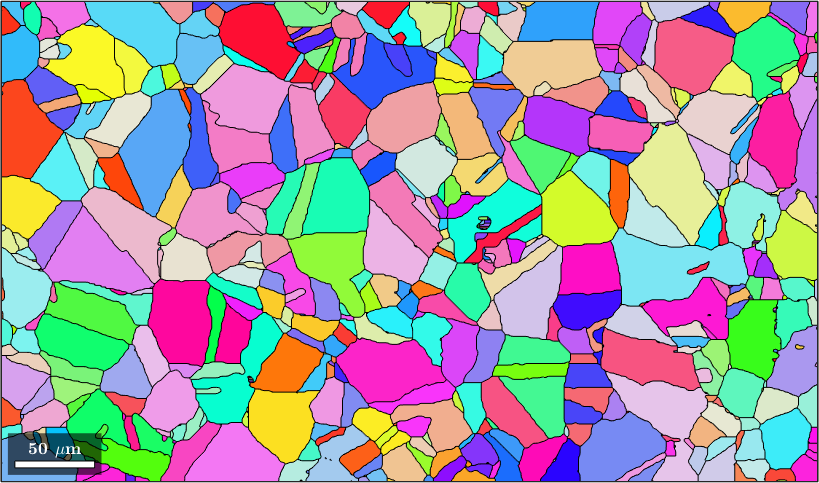
Next we plot image quality as it makes the grain boundaries visible. and overlay it with the orientation map
plot(ebsd,log(ebsd.prop.iq),'figSize','large')
mtexColorMap black2white
setColorRange([.5,5])

% the option 'FaceAlpha',0.4 makes the plot a bit translucent
hold on
plot(grains,grains.meanOrientation,'FaceAlpha',0.4,'linewidth',3)
hold off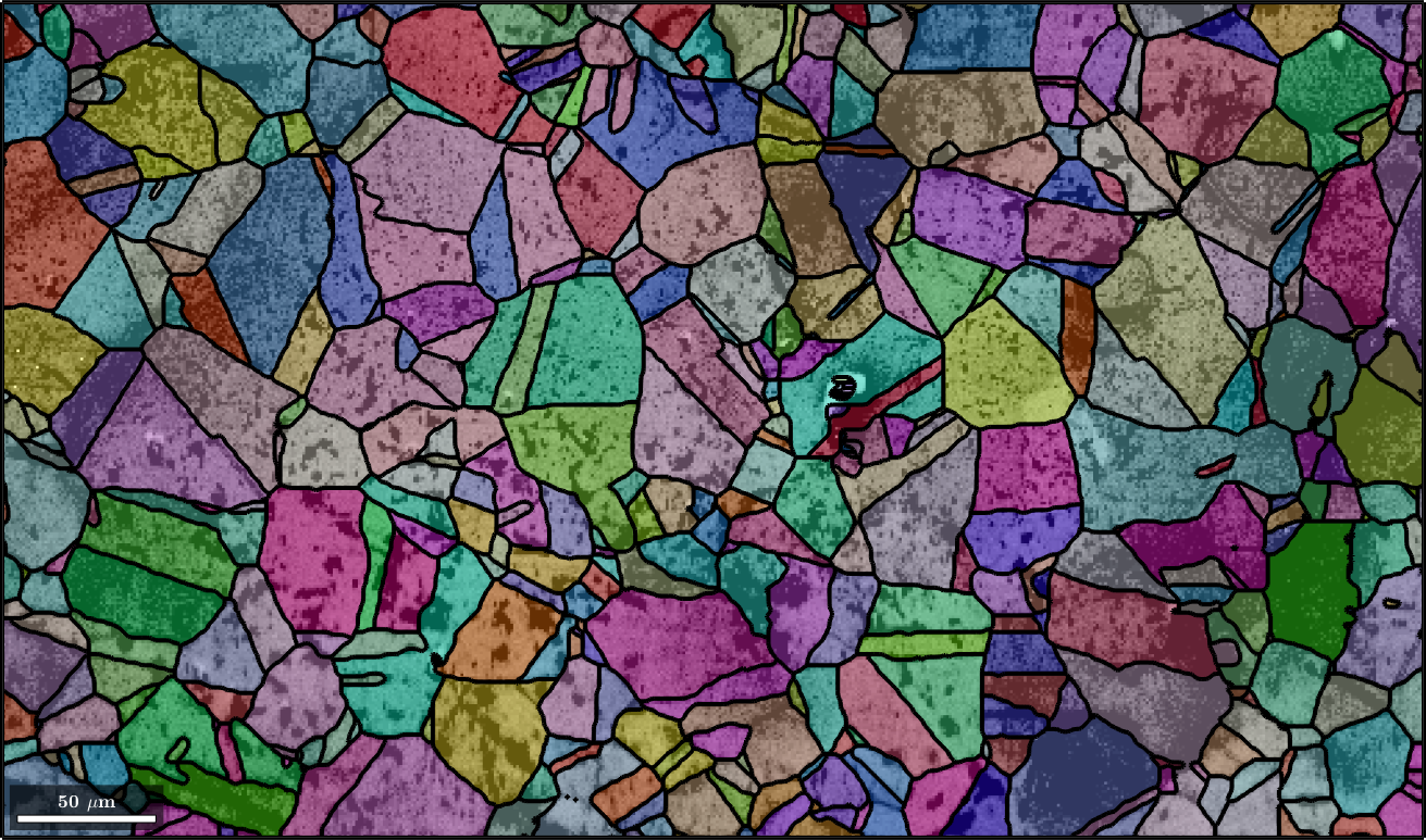
Detecting CSL Boundaries
In order to detect CSL boundaries within the data set we first restrict the grain boundaries to iron to iron phase transitions and check then the boundary misorientations to be a CSL(3) misorientation with threshold of 3 degree.
% restrict to iron to iron phase transition
gB = grains.boundary('iron','iron')

% select CSL(3) grain boundaries
gB3 = gB(angle(gB.misorientation,CSL(3,ebsd.CS)) < 3*degree);

% overlay CSL(3) grain boundaries with the existing plot
hold on
plot(gB3,'lineColor','gold','linewidth',3,'DisplayName','CSL 3')
hold off
gB = grainBoundary
Segments length mineral 1 mineral 2
20356 16362 µm iron iron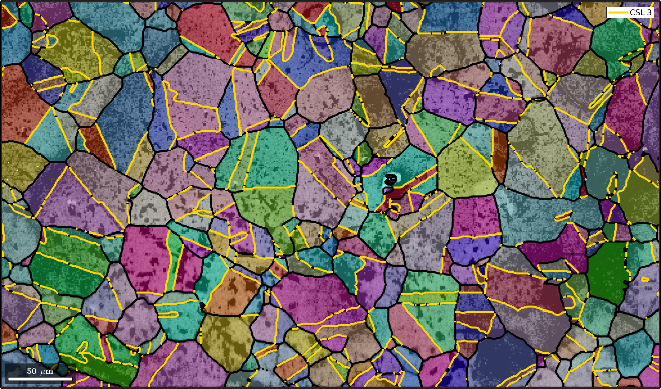
Mark triple points
Next we want to mark all triple points with at least 2 CSL boundaries
% logical list of CSL boundaries
isCSL3 = grains.boundary.isTwinning(CSL(3,ebsd.CS),3*degree);

% logical list of triple points with at least 2 CSL boundaries
tPid = sum(isCSL3(grains.triplePoints.boundaryId),2)>=2;

% plot these triple points
hold on
plot(grains.triplePoints(tPid),'color','red','linewidth',2,'MarkerSize',8)
hold off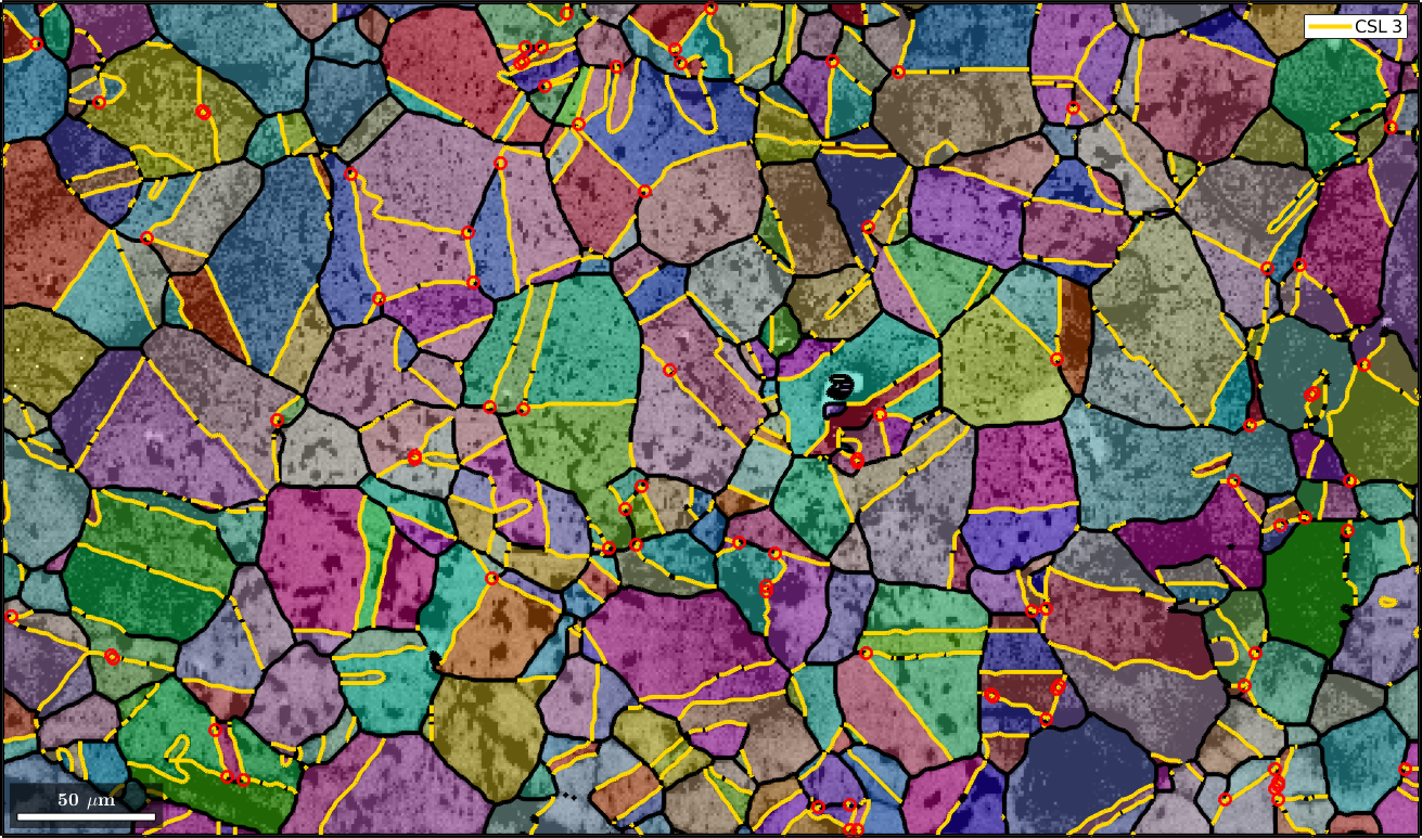
Merging grains with common CSL(3) boundary
Next we merge all grains together which have a common CSL(3) boundary. This is done with the command merge.
% this merges the grains
[mergedGrains,parentIds] = merge(grains,gB3);

% overlay the boundaries of the merged grains with the previous plot
hold on
plot(mergedGrains.boundary,'linecolor','w','linewidth',3)
hold off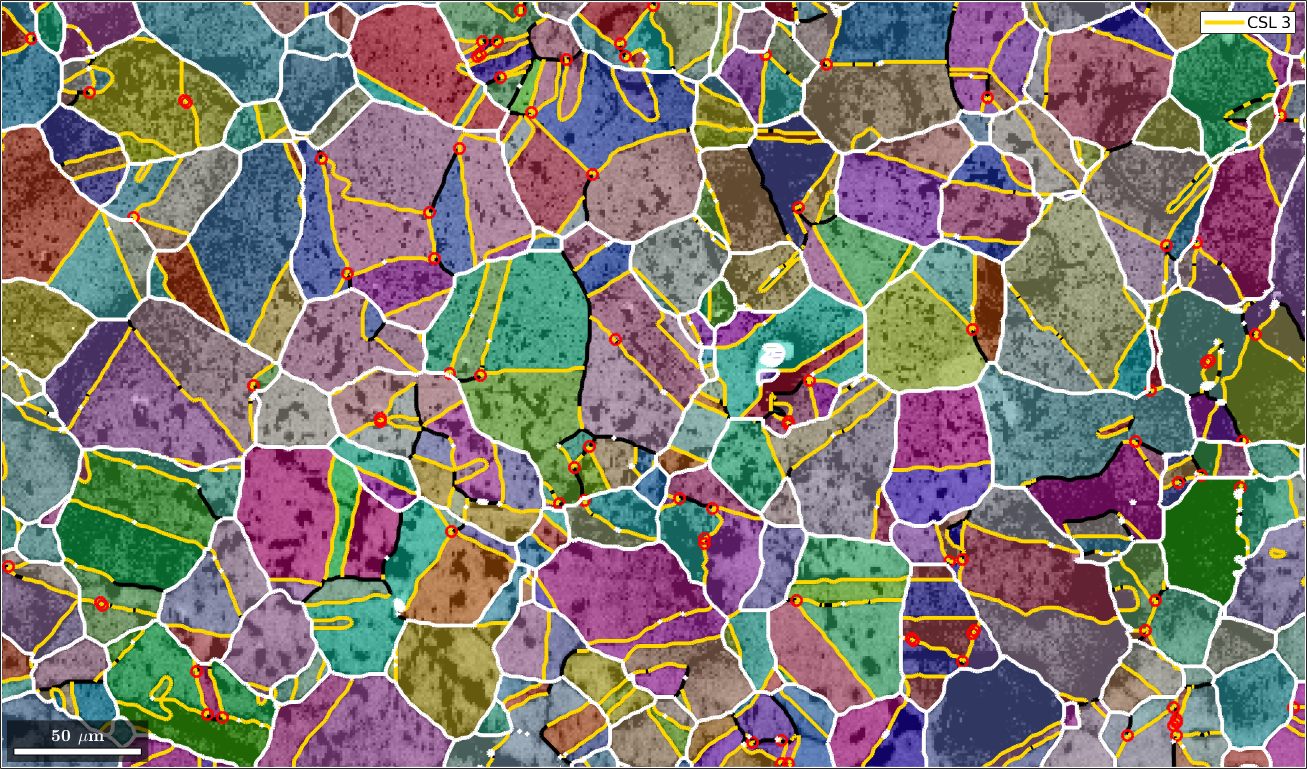
Finaly, we check for all other types of CSL boundaries and overlay them with our plot.
delta = 5*degree;
gB5 = gB(gB.isTwinning(CSL(5,ebsd.CS),delta));
gB7 = gB(gB.isTwinning(CSL(7,ebsd.CS),delta));
gB9 = gB(gB.isTwinning(CSL(9,ebsd.CS),delta));
gB11 = gB(gB.isTwinning(CSL(11,ebsd.CS),delta));

hold on
plot(gB5,'lineColor','b','linewidth',2,'DisplayName','CSL 5')
hold on
plot(gB7,'lineColor','g','linewidth',2,'DisplayName','CSL 7')
hold on
plot(gB9,'lineColor','m','linewidth',2,'DisplayName','CSL 9')
hold on
plot(gB11,'lineColor','c','linewidth',2,'DisplayName','CSL 11')
hold off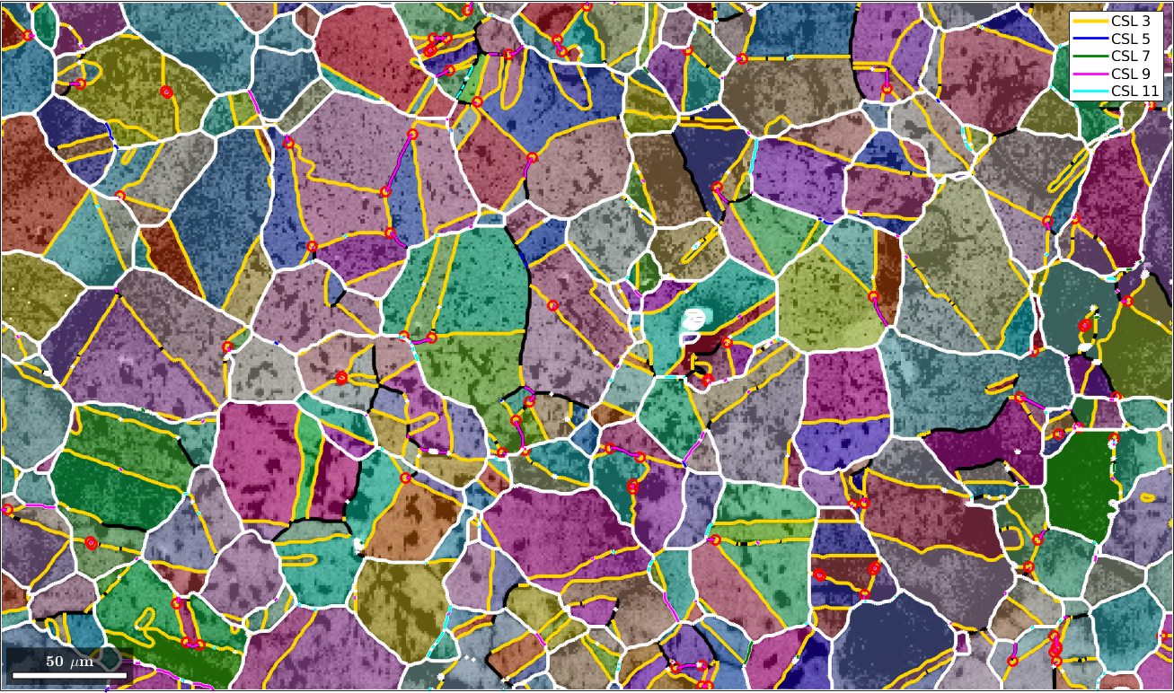
Misorientations in the 3d fundamental zone
We can also look at the boundary misorientations in the 3 dimensional fundamental orientation zone.
% compute the boundary of the fundamental zone
oR = fundamentalRegion(ebsd.CS,ebsd.CS,'antipodal');
close all
plot(oR)

% plot 500 random misorientations in the 3d fundamental zone
mori = discreteSample(gB.misorientation,500);
hold on
plot(mori.project2FundamentalRegion)
hold off

% mark the CSL(3) misorientation
hold on
csl3 = CSL(3,ebsd.CS);
plot(csl3.project2FundamentalRegion('antipodal') ,'MarkerColor','r','DisplayName','CSL 3','MarkerSize',20)
hold off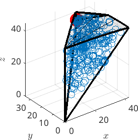
Analyzing the misorientation distribution function
In order to analyze more quantitatively the boundary misorientation distribution we can compute the so called misorientation distribution function. The option antipodal is applied since we want to identify mori and inv(mori).
mdf = calcDensity(gB.misorientation,'halfwidth',5*degree,'bandwidth',48)mdf = SO3FunHarmonic (iron → iron)
antipodal: true
bandwidth: 48
weight: 1Next we can visualize the misorientation distribution function in axis angle sections.
plot(mdf,'axisAngle',(25:5:60)*degree,'colorRange',[0 15])

annotate(CSL(3,ebsd.CS),'label','\(CSL_3\)','backgroundcolor','w')
annotate(CSL(5,ebsd.CS),'label','\(CSL_5\)','backgroundcolor','w')
annotate(CSL(7,ebsd.CS),'label','\(CSL_7\)','backgroundcolor','w')
annotate(CSL(9,ebsd.CS),'label','\(CSL_9\)','backgroundcolor','w')

drawNow(gcm)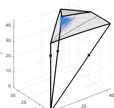
The MDF can be now used to compute preferred misorientations
[~,mori] = max(mdf,'numLocal',2)mori = misorientation (iron → iron)
size: 2 x 1
antipodal: true
Bunge Euler angles in degree
phi1 Phi phi2
116.493 48.1916 206.647
103.655 26.4436 283.461and their volumes in percent
100 * volume(gB.misorientation,CSL(3,ebsd.CS),2*degree)

100 * volume(gB.misorientation,CSL(9,ebsd.CS),2*degree)
ans =
40.9904
ans =
2.0338or to plot the MDF along certain fibers
omega = linspace(0,60*degree);
fibre100 = orientation.byAxisAngle(xvector,omega,mdf.CS,mdf.SS)
fibre111 = orientation.byAxisAngle(vector3d(1,1,1),omega,mdf.CS,mdf.SS)
fibre101 = orientation.byAxisAngle(vector3d(1,0,1),omega,mdf.CS,mdf.SS)

close all
plot(omega ./ degree,mdf.eval(fibre100),'LineWidth',2)
hold on
plot(omega ./ degree,mdf.eval(fibre111),'LineWidth',2)
plot(omega ./ degree,mdf.eval(fibre101),'LineWidth',2)
hold off
legend('100','111','101')
xlabel('misorientation angle');
ylabel('mrd');
fibre100 = misorientation (iron → iron)
size: 1 x 100
fibre111 = misorientation (iron → iron)
size: 1 x 100
fibre101 = misorientation (iron → iron)
size: 1 x 100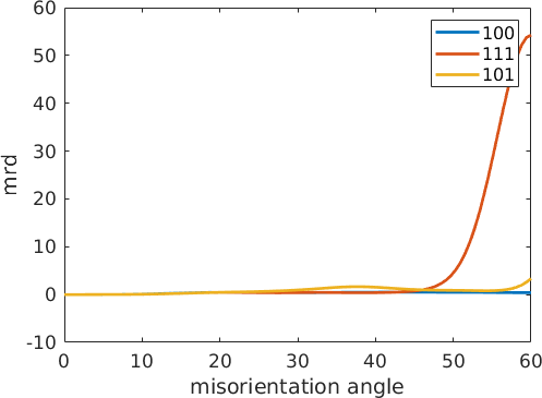
or to evaluate it in an misorientation directly
mori = orientation.byEuler(15*degree,28*degree,14*degree,mdf.CS,mdf.CS)

mdf.eval(mori)

mdf.eval(csl3)
mori = misorientation (iron → iron)
Bunge Euler angles in degree
phi1 Phi phi2
15 28 14
ans =
1.5276
ans =
54.2486