Exporting figures

Export is the last step of making a figure. Add its colour scale, labels, and other reading aids first, then choose a file type that suits the plotted objects. Dense spatial maps usually belong in a bitmap. Lines, markers, and text usually benefit from a vector format.

Every MTEX figure is an ordinary MATLAB figure. You can export it through File / Save As or with MATLAB's print and exportgraphics commands. These routes usually leave a broad white margin around an MTEX plot. On a spatial EBSD map, they may also interpolate between neighbouring pixels. That interpolation can invent colours which are absent from the data.

saveFigure handles these details for MTEX figures and produces cropped, publication-ready files. Complete the workflow from Annotations before calling it.

A first export

Start with an orientation map. Each coloured cell is one measurement, so an exported bitmap must keep neighbouring cell colours discrete. This is a case where preserving the values matters more than making cell boundaries look smooth.

plottingConvention.default('y↑→x');
mtexdata forsterite silent

ebsdF = ebsd('Forsterite');
plot(ebsdF,ebsdF.orientations)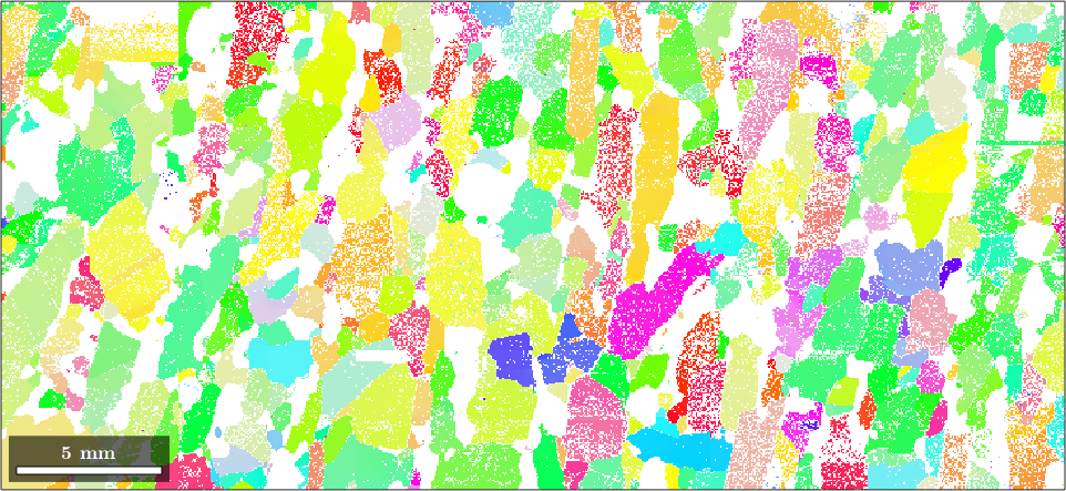

Notice the sharp changes of colour between neighbouring measurements. The exported image should retain those changes rather than blend across them.

The filename extension determines the output format. The vector formats are pdf, eps, and ps. The bitmap formats are png, jpg, tif, and bmp. saveFigure overwrites an existing file with the same name, so choose the output path deliberately. Check that the file you asked for exists before relying on it, as the next step does.

% write into a temporary folder rather than the MTEX folder
outDir = fullfile(tempdir,'mtex-docrun','scratch');
if ~isfolder(outDir), mkdir(outDir); end
outMap = fullfile(outDir,'forsterite.png');

saveFigure(outMap)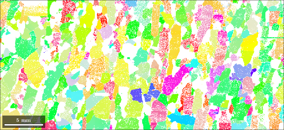

Confirm that the export produced a file before using it elsewhere. The assertion remains silent when it succeeds. It stops the page if exporting failed.

assert(isfile(outMap),'The orientation-map export was not created.')

Vector graphics and bitmaps

A vector file stores drawn objects as paths and text. A bitmap stores a fixed grid of coloured pixels. saveFigure treats the two groups differently. Choose a vector file when paths and text should remain sharp at any magnification. Choose a bitmap when the figure contains many cells or patches and a compact, fixed-resolution image is preferable.

Vector formats are written by print. Before printing, saveFigure sets the paper size to the figure size. The resulting page is exactly as large as the plot and has no broad margin. When necessary, saveFigure switches the renderer to painters mode because painters produces true vector output. A spatial EBSD map contains one patch per measurement. It can therefore make a very large vector file, so a bitmap is usually the better choice for maps.

Bitmap formats are written by export_fig at 1.5 times the screen resolution. For a spatial map, MTEX increases the factor to 2.5 and turns graphics smoothing off. This prevents new colours from being introduced between map cells. It matters when orientations will be read back from their colour.

Two options are passed to the underlying tools.

Both options call programs from a TeX distribution. They are available only on Unix-like systems. Without those external programs, export directly to the required extension and omit the two options.

Controlling output size

Bitmap resolution follows the on-screen figure size. The output is enlarged internally by the factors above, but its proportions still come from that figure. To obtain a larger or smaller image, create a larger or smaller figure with 'figSize' before exporting it.

plot(ebsdF,ebsdF.orientations,'figSize','small')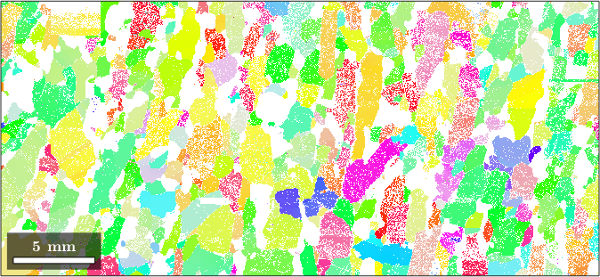

This map uses a smaller canvas than the first map. Saving it now would therefore produce a smaller bitmap with the same map content.

The recognized values are 'tiny', 'small', 'normal', 'large' and 'huge', and they are relative to the screen size. The default is stored as an MTEX preference and can be changed permanently by setMTEXpref('figSize','large'). For a one-off export, passing 'figSize' to the plot keeps the choice local to that figure.

For a multi-plot, 'figSize' refers to each panel rather than to the whole figure. Three pole figures at 'normal' therefore give three panels the size of a single normal-sized plot.

plotPDF(ebsdF.orientations,...
  Miller({1,0,0},{0,1,0},{0,0,1},ebsdF.CS),...
  'contourf','figSize','normal')
mtexColorbar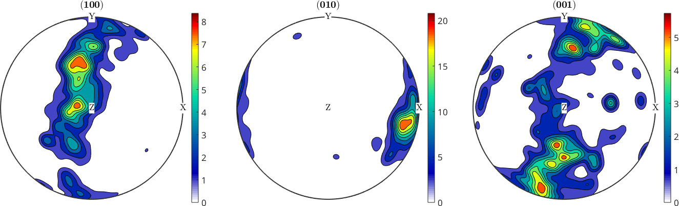

The figure is three times as wide as a single pole figure, while each panel keeps the size it would have on its own. Increasing 'figSize' enlarges every panel and the figure with them. Export the complete figure as a bitmap and verify the file just as for the map.

outPole = fullfile(outDir,'poleFigures.png');
saveFigure(outPole)
assert(isfile(outPole),'The pole-figure export was not created.')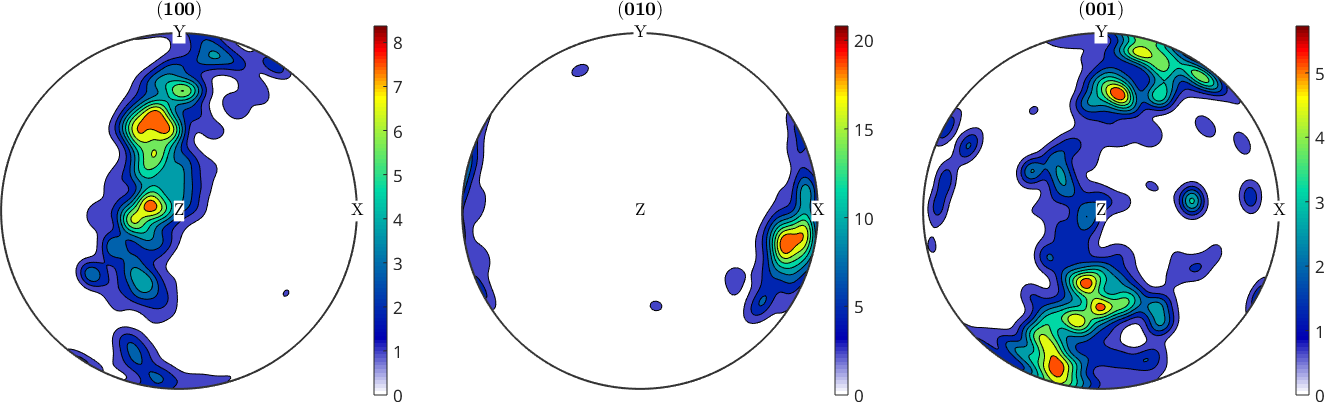

Exporting data instead of a picture

A figure file stores the visual result, not the numerical values behind it. When those values are the required result, use a class-specific export method instead. Most MTEX classes provide one. Examples are export for orientations, export for pole-figure data, and export for ODFs. Their corresponding chapters describe the data formats. This distinction avoids treating pixels in a saved picture as though they were the original measurements.

% clean up
delete(outMap)
delete(outPole)

References

Next

Export completes the figure workflow. Continue with Spherical Projections to understand how the projection itself changes the positions, shapes, and areas seen in pole figures and other spherical plots.

References

- O. Woodford and Y. Altman,
export_fig, open-source MATLAB software, 2008--present, provides the bitmap-export backend used bysaveFigure.