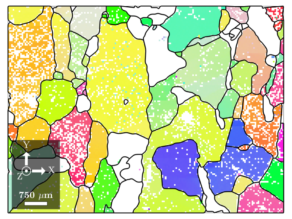
Your first EBSD analysis

Code

mtexdata forsterite silent
ebsd = ebsd(inpolygon(ebsd,[12000 3000 9000 6750]));
grains = smoothBoundary(calcGrains(ebsd,'angle',10*degree,'minPixel',5),5);
plot(ebsd('Forsterite'),ebsd('Forsterite').orientations)
hold on, plot(grains.boundary,'lineWidth',1.5), hold off

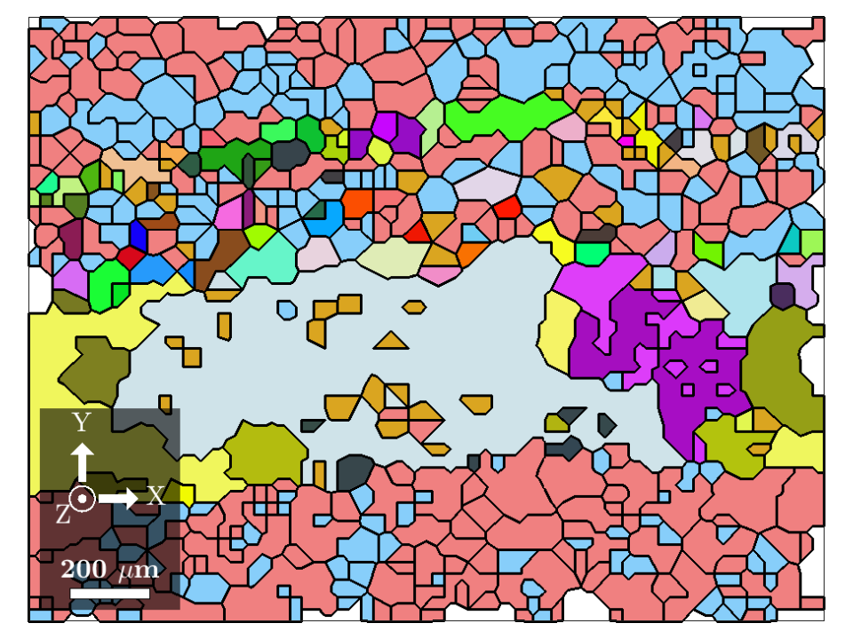
Your first grain analysis

Code

mtexdata mylonite silent
ebsd = ebsd(inpolygon(ebsd,[21000 1500 2000 1500]));
[grains,ebsd] = calcGrains(ebsd,'angle',15*degree);
plot(grains)
hold on
plot(grains('Quartz'),grains('Quartz').meanOrientation)
plot(grains.boundary,'lineWidth',1.5)
hold off

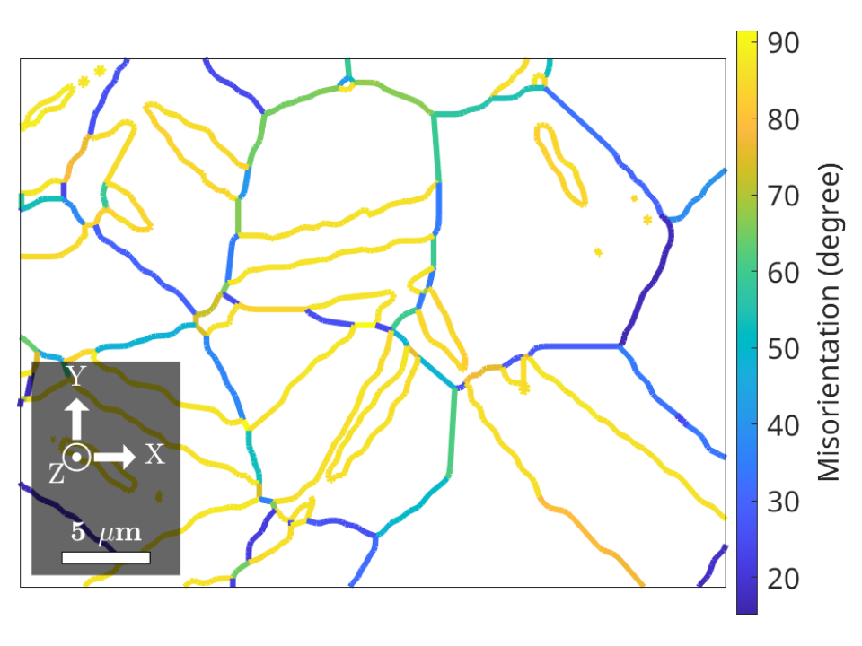
Your first boundary analysis

Code

mtexdata twins silent
grains = smoothBoundary(calcGrains(ebsd,'angle',15*degree),5);
gB = grains.boundary('Magnesium','Magnesium');
plot(gB,gB.misorientation.angle./degree,'lineWidth',3)
mtexColorbar('title','Misorientation (degree)')

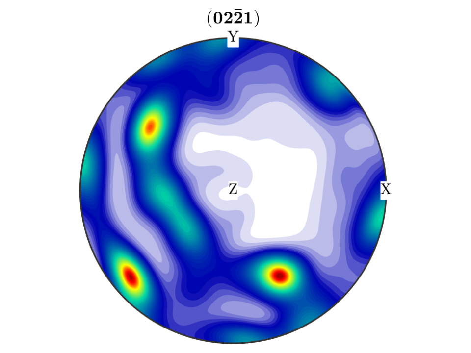
Your first pole figure analysis

Code

mtexdata dubna silent
odf = calcODF(pf,'silent');
plotPDF(odf,pf.allH(1),'antipodal')

Your first texture analysis

Code

mtexdata titanium silent
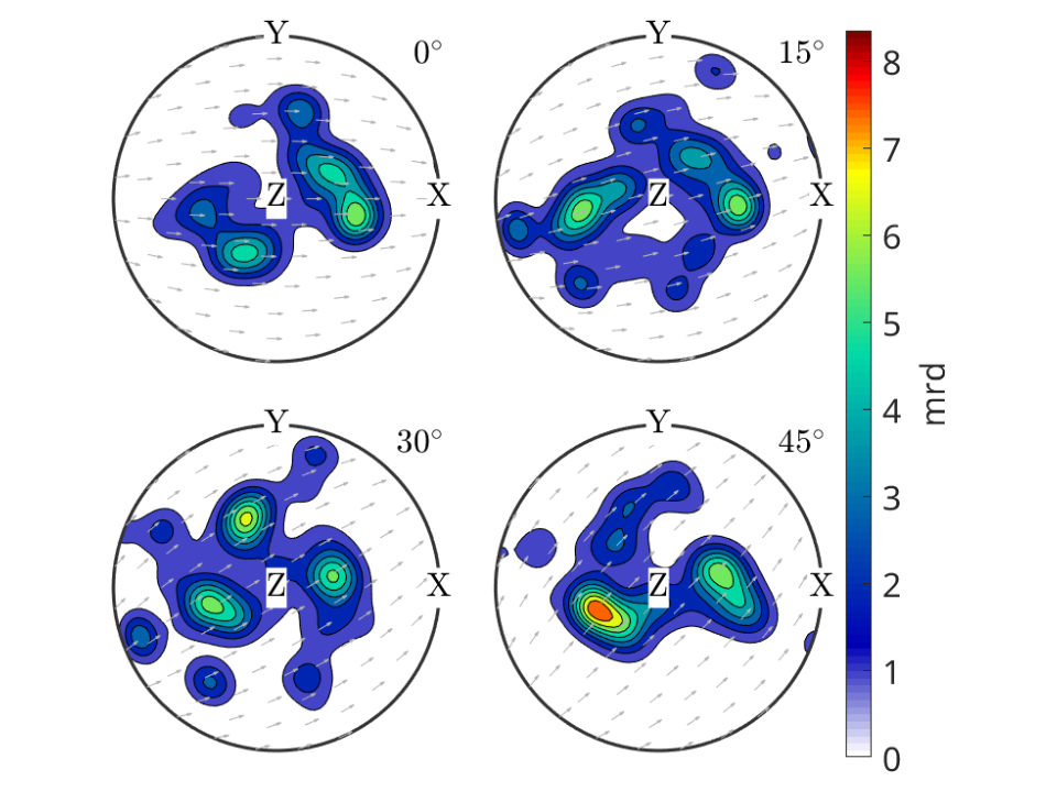
odf = calcDensity(ebsd('Titanium (Alpha)').orientations,'halfwidth',10*degree);
plotSection(odf,'sigma','sections',4,'contourf')
mtexColorbar('title','mrd')

Colouring EBSD maps

Code

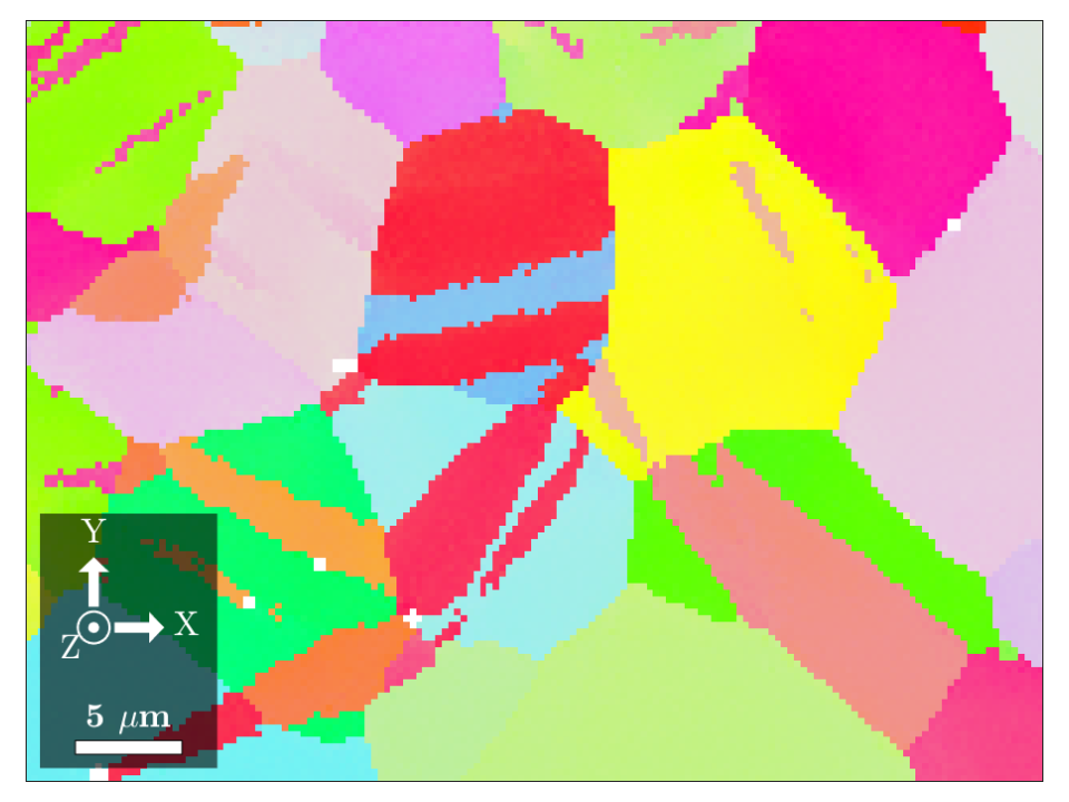
mtexdata twins silent
plot(ebsd,'ipfDirection',zvector)

Twin boundaries

Code

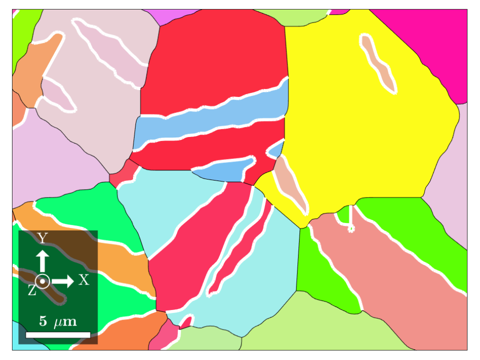
[grains,ebsd] = calcGrains(ebsd,'angle',5*degree,'minPixel',3);
grains = smoothBoundary(grains,5);
twin = orientation.map(Miller(1,-1,0,1,grains.CS),Miller(1,0,-1,-1,grains.CS),...
  Miller(0,1,-1,1,grains.CS,'uvw'),Miller(1,-1,0,1,grains.CS,'uvw'));
gB = grains.boundary('Magnesium','Magnesium');
twinB = gB(gB.isTwinning(twin,5*degree));
plot(grains,grains.meanOrientation,'ipfDirection',zvector), hold on
plot(twinB,'lineColor','w','lineWidth',3), hold off

Boundary misorientations

Code

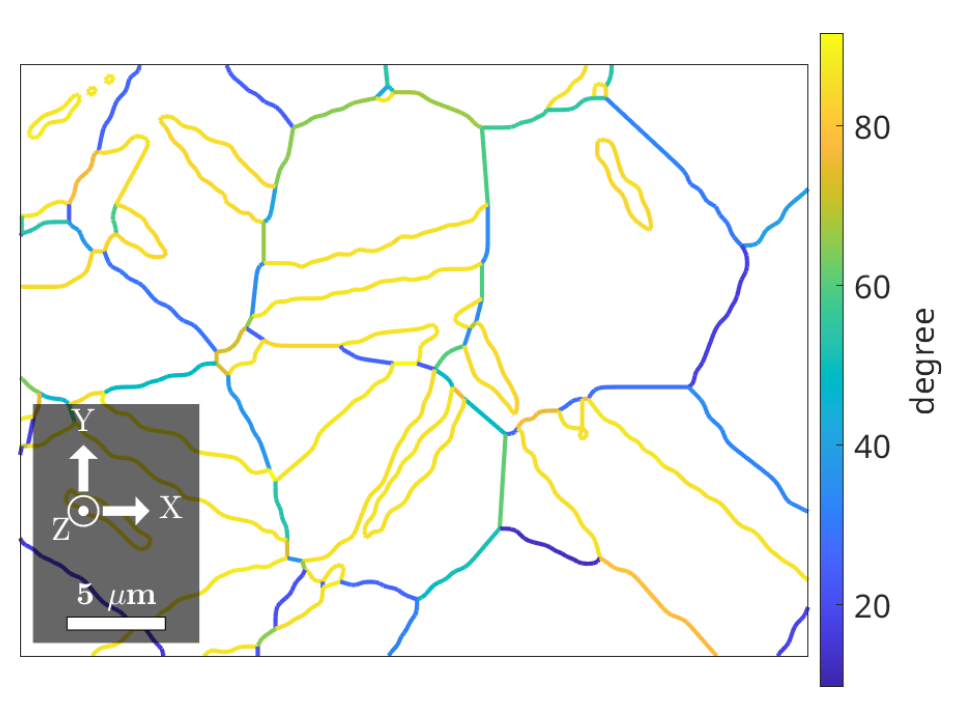
plot(gB,gB.misorientation.angle./degree,'lineWidth',2)
mtexColorbar('title','degree')

Misorientation distributions

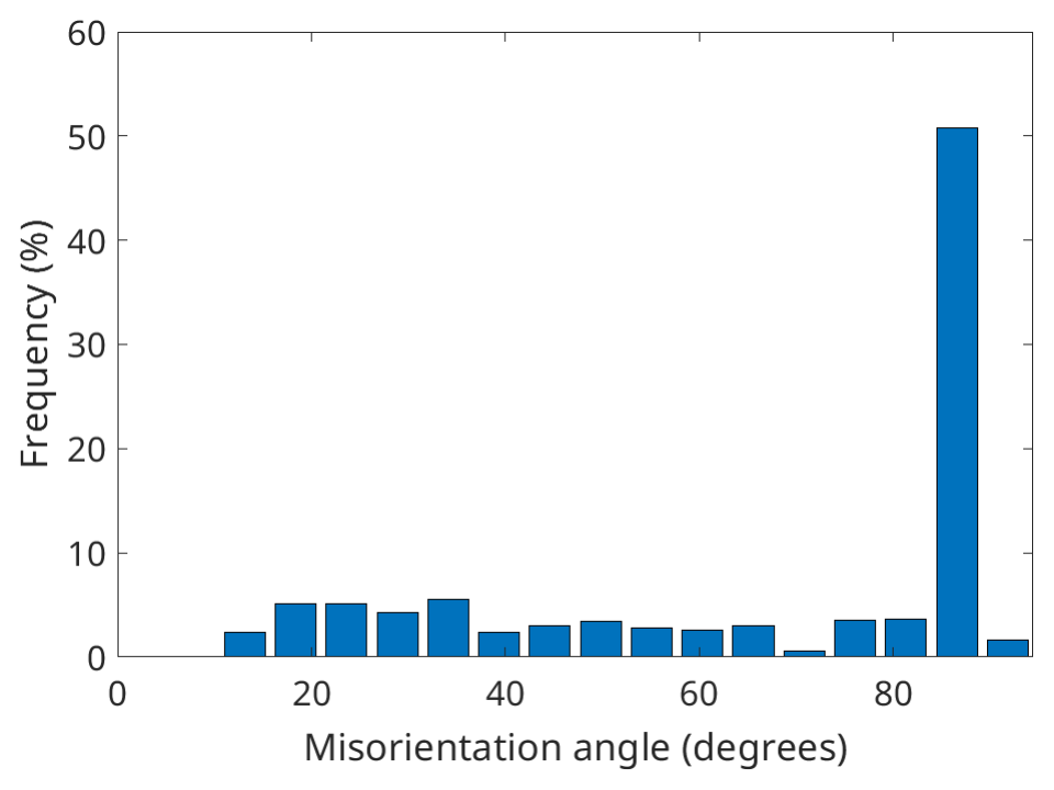
Code

plotAngleDistribution(gB.misorientation)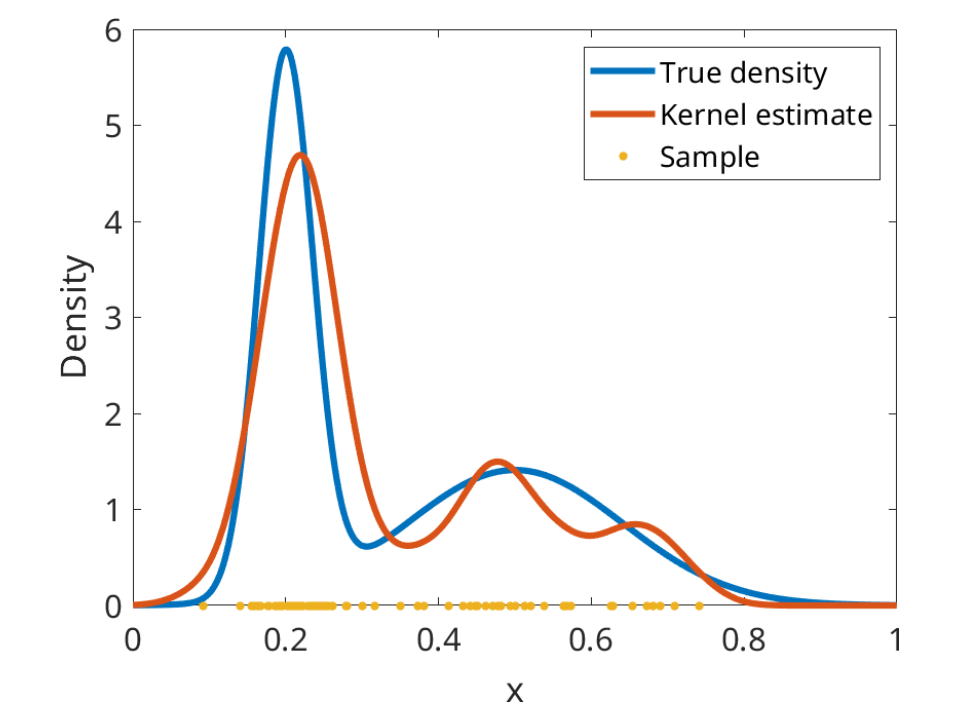

Density estimation

Code

x = linspace(0,1,500);
f = @(x) (Gaussian(0.2,0.05,x)+Gaussian(0.5,0.2,x))/2;
sample = discreteSample(f,80,'range',[0 1]);
psi = Gaussian(0,0.05);
estimate = @(x) mean(psi(x-sample),1);
plot(x,f(x),'lineWidth',3), hold on
plot(x,estimate(x),'lineWidth',3)
plot(sample,zeros(size(sample)),'.','markerSize',14)
hold off
legend('True density','Kernel estimate','Sample','Location','northeast')
xlabel('x'), ylabel('Density')

Spherical density estimation

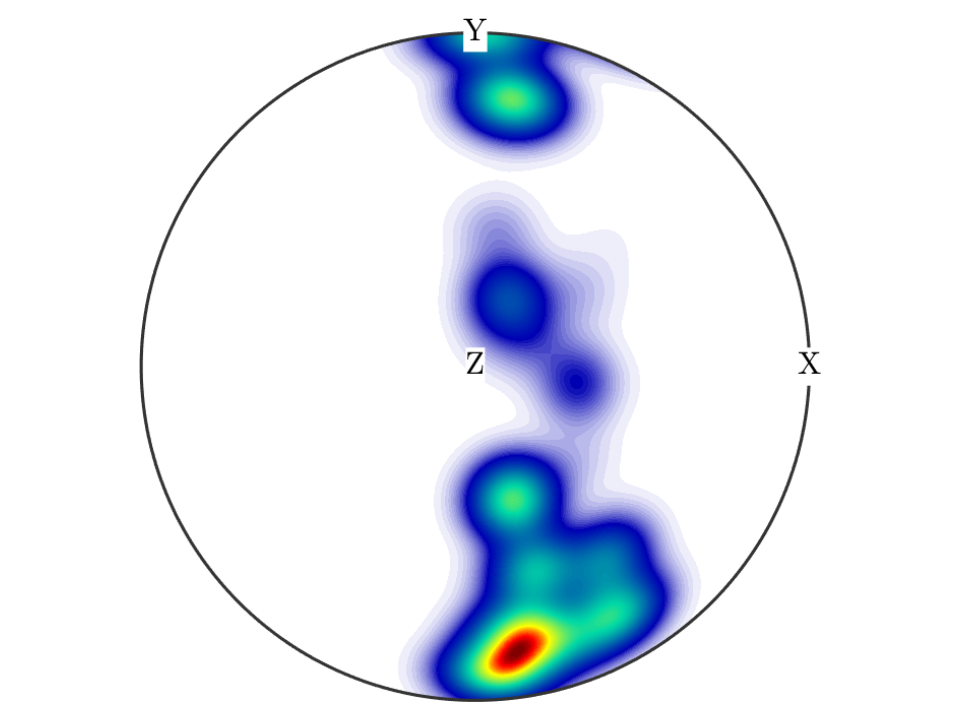
Code

c = ebsd('Magnesium').orientations * Miller(0,0,0,1,ebsd('Magnesium').CS);
plot(calcDensity(c,'halfwidth',7.5*degree),'upper')

Kernel average misorientation

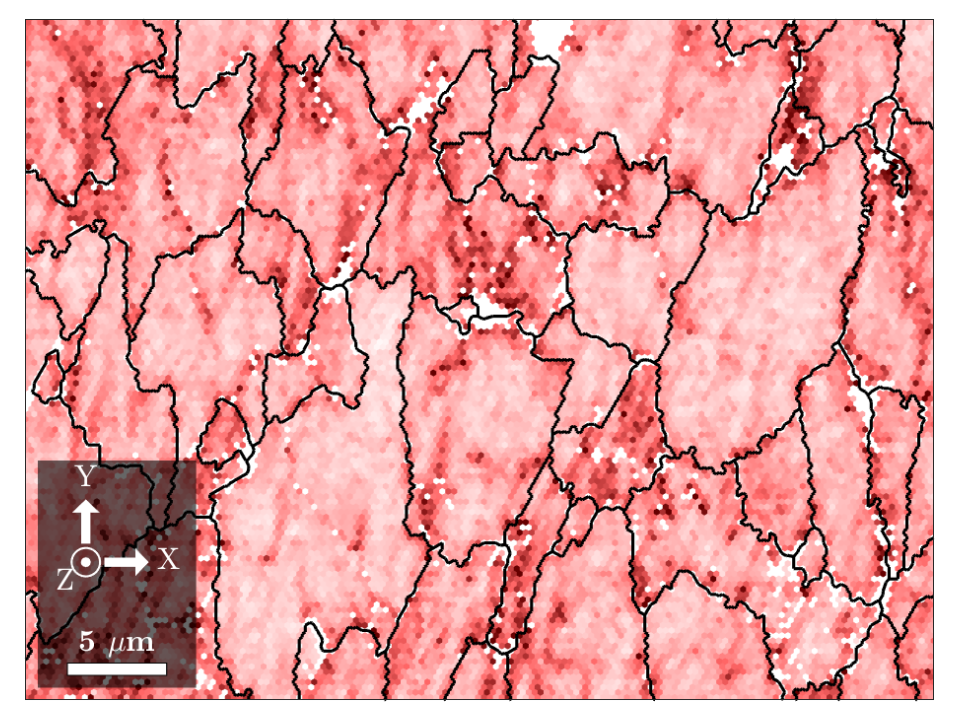
Code

mtexdata ferrite
[grains,ebsd] = calcGrains(ebsd,'minPixel',8);
plot(ebsd,ebsd.KAM('threshold',2.5*degree)./degree)
setColorRange([0 2]), mtexColorMap LaboTeX
hold on, plot(grains.boundary,'lineWidth',1.5), hold off

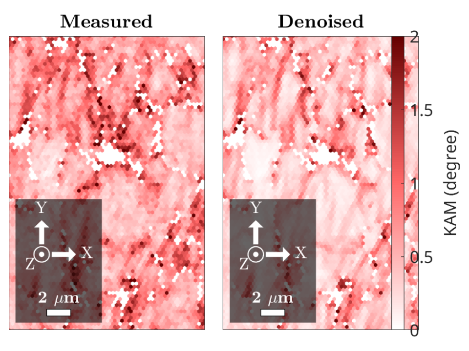
Denoising orientation maps

Code

ebsdS = smooth(ebsd('indexed'),l1TVFilter);
newMtexFigure('layout',[1 2]);
plot(ebsd,ebsd.KAM('threshold',2.5*degree)./degree)
mtexTitle('Measured')
nextAxis
plot(ebsdS,ebsdS.KAM('threshold',2.5*degree)./degree)
mtexTitle('Denoised')
setColorRange([0 2]), mtexColorMap LaboTeX
mtexColorbar('title','KAM (degree)')

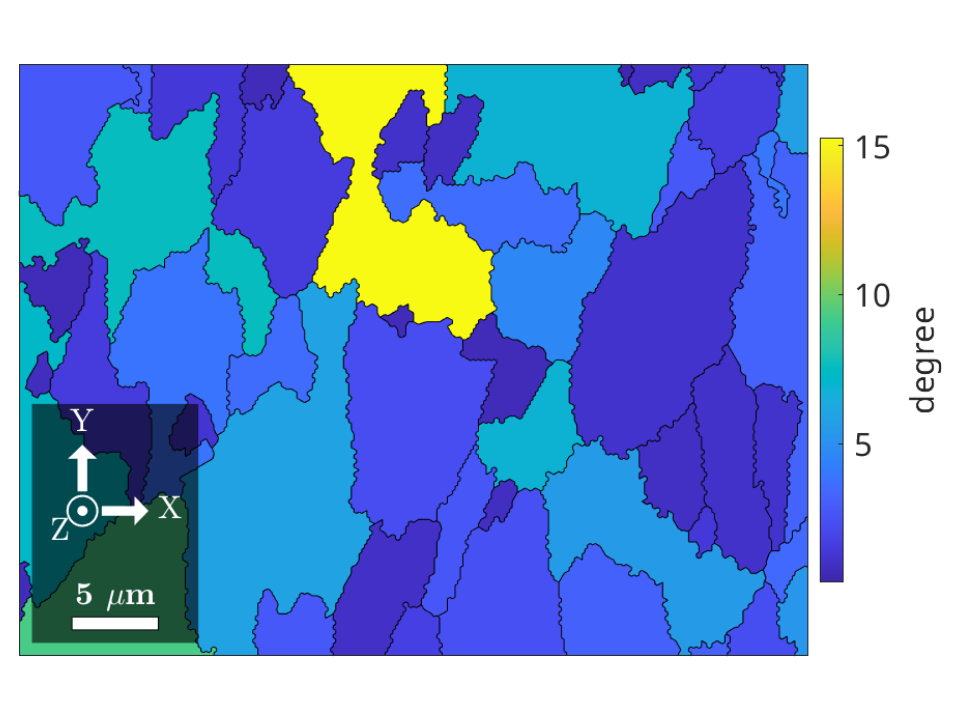
Grain orientation parameters

Code

mis2mean = calcGROD(ebsd,grains);
GOS = ebsd.grainMean(mis2mean.angle,grains);
plot(grains,GOS./degree)
mtexColorbar('title','degree')

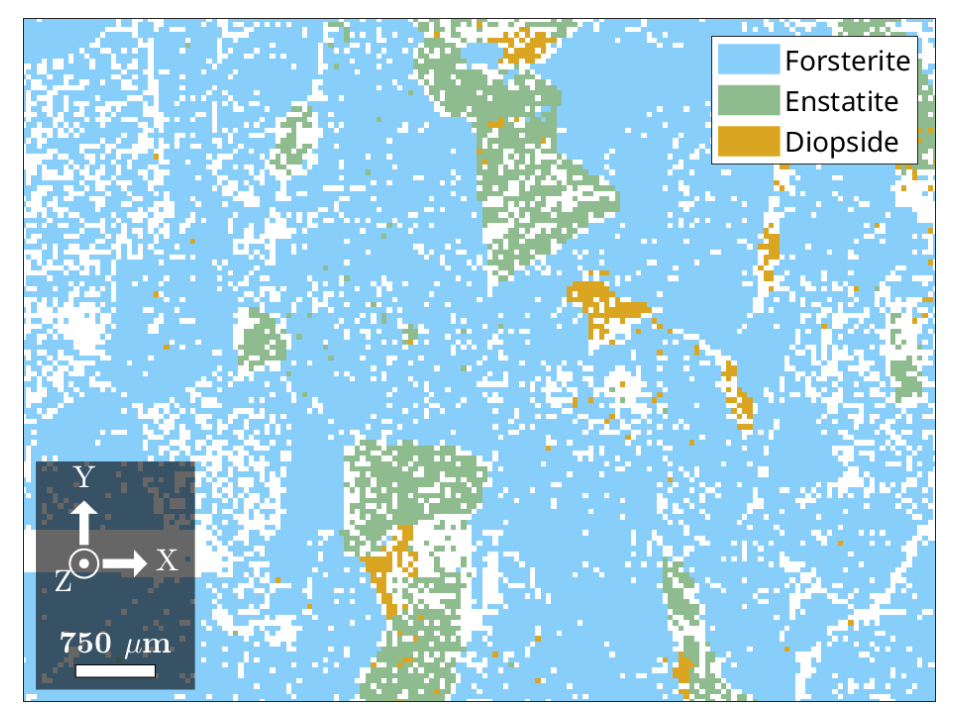
Phase maps

Code

mtexdata forsterite
ebsd = ebsd(inpolygon(ebsd,[12000 3000 9000 6750]));
plot(ebsd)

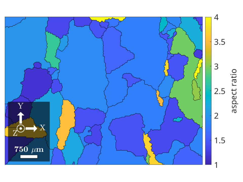
Grain shape parameters

Code

grains = calcGrains(ebsd,'minPixel',10);
plot(grains,grains.aspectRatio)
setColorRange([1 4]), mtexColorbar('title','aspect ratio')

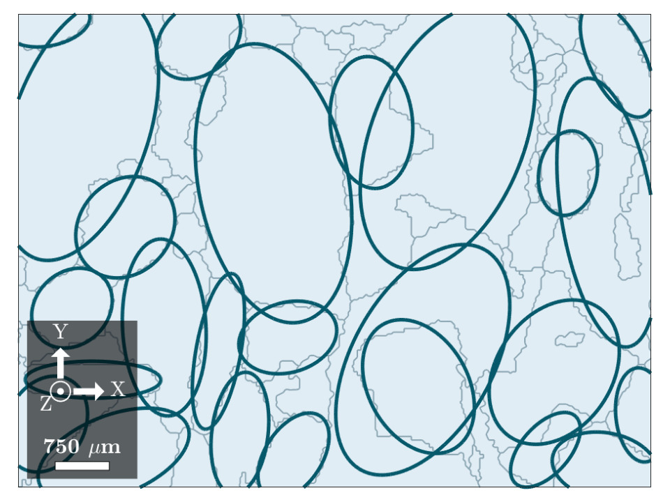
Ellipse fitting

Code

[c,a,b] = grains(grains.numPixel>200).fitEllipse;
plot(grains,'faceColor',[0.88 0.93 0.96]), hold on
plot(grains.boundary,'lineWidth',1,'lineColor',[0.55 0.65 0.7])
plotEllipse(c,a,b,'lineColor',[0.02 0.35 0.42],'lineWidth',2.5), hold off

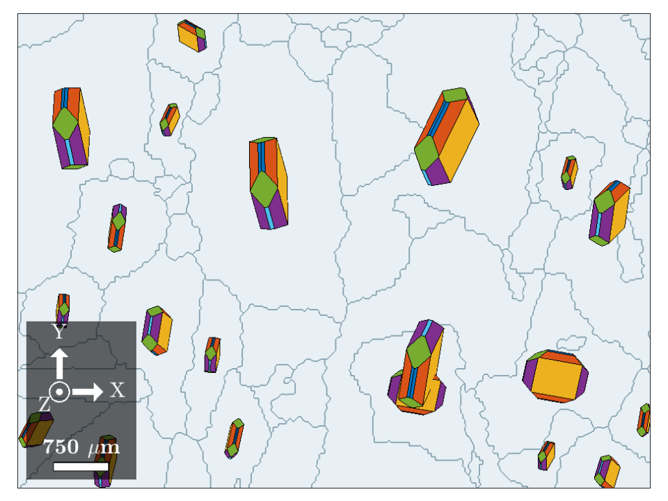
Crystal shapes

Code

fo = grains('Forsterite');
[~,id] = sort(fo.area,'descend');
cS = crystalShape.olivine(fo.CS);
plot(grains,'faceColor',[0.91 0.94 0.96]), hold on
plot(grains.boundary,'lineWidth',1,'lineColor',[0.55 0.65 0.7])
plot(fo(id(1:min(20,numel(id)))),0.55*cS,'colored'), hold off

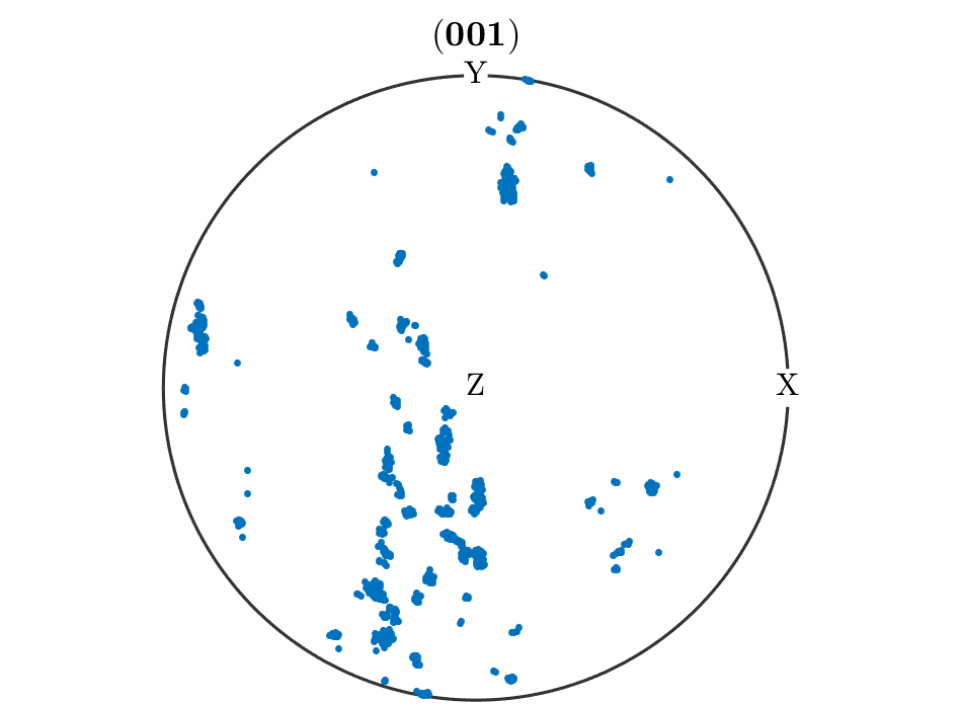
Pole figures

Code

ori = ebsd('Forsterite').orientations;
plotPDF(ori,Miller(0,0,1,ori.CS),'points',5000,'markerSize',3)

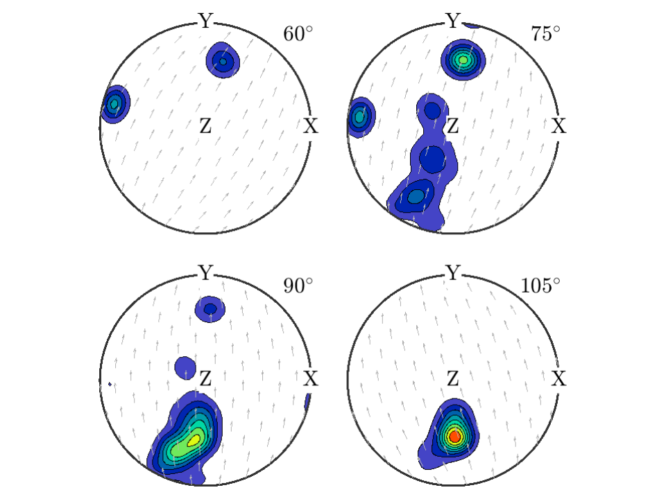
ODF sections

Code

odf = calcDensity(ori);
plotSection(odf,'sigma',(60:15:105)*degree,'contourf')

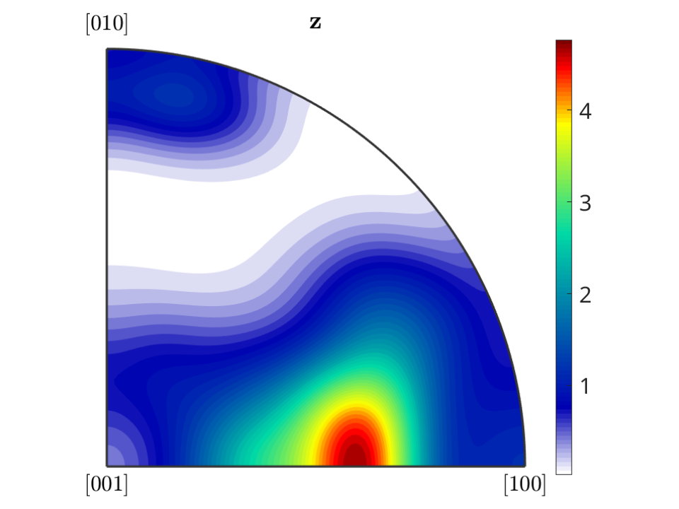
Inverse pole figures

Code

plotIPDF(odf,zvector)
mtexColorbar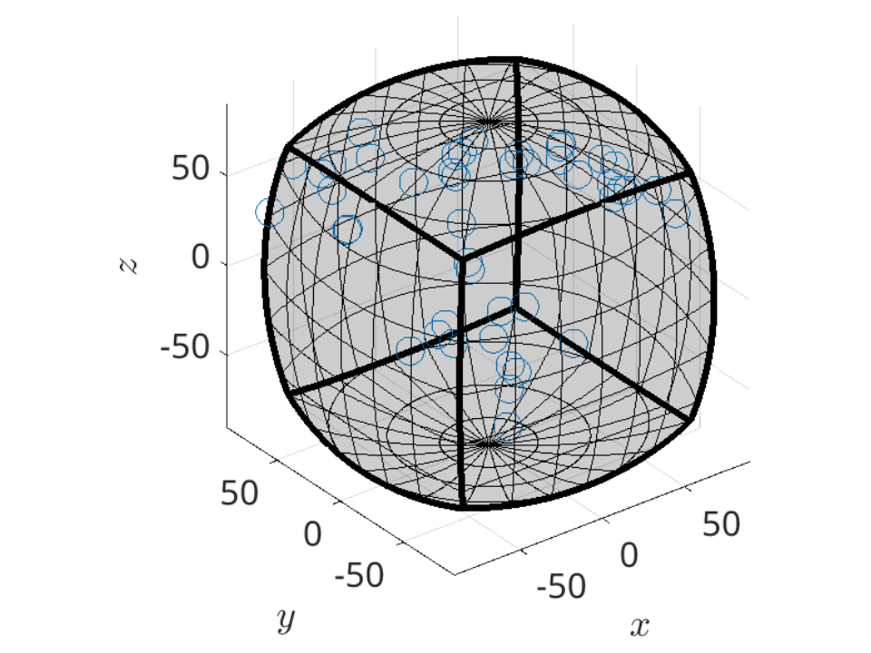

Fundamental regions

Code

plot(grains('Forsterite').meanOrientation,'axisAngle','markerSize',12)

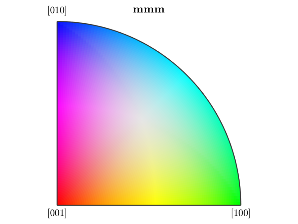
Colour keys

Code

plot(ipfColorKey(ebsd('Forsterite')))

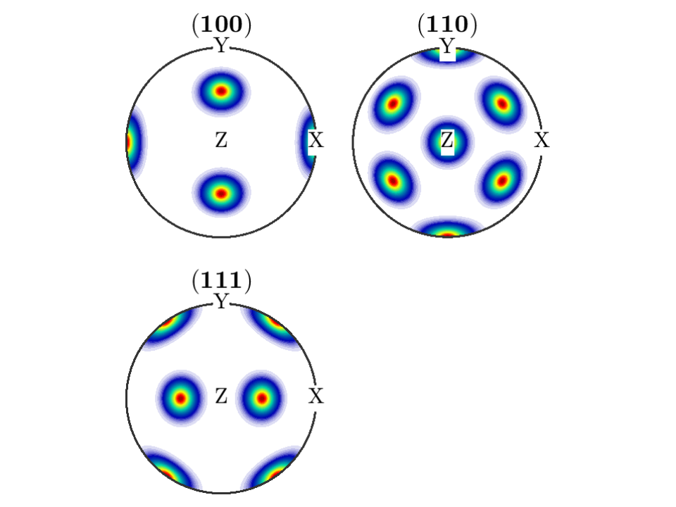
Model textures

Code

cs = crystalSymmetry('m-3m');
odf = unimodalODF(orientation.goss(cs),'halfwidth',10*degree);
plotPDF(odf,Miller({1,0,0},{1,1,0},{1,1,1},cs),'layout',[2 2])

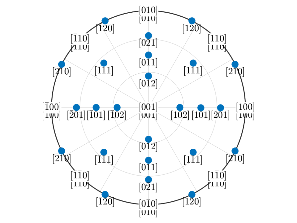
Miller indices

Code

m = Miller({1,0,0},{1,1,0},{1,1,1},{2,1,0},cs,'uvw');
plot(m,'symmetrised','labeled','upper','grid')

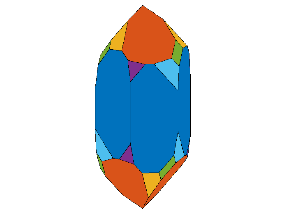
Crystal morphology

Code

plot(crystalShape.quartz,'colored')

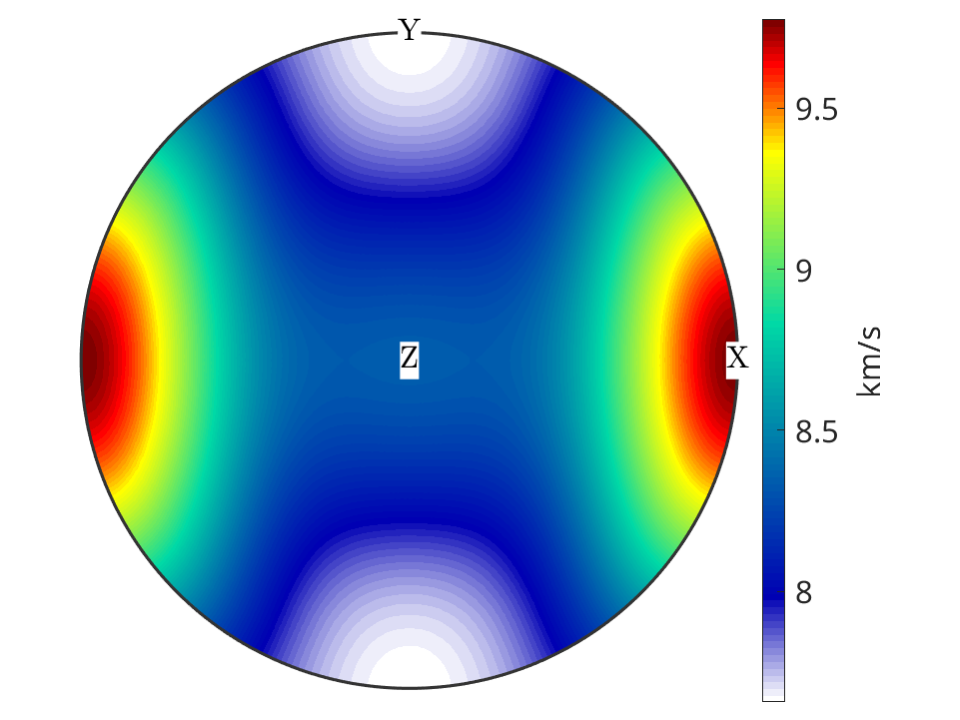
Wave velocities

Code

cs = crystalSymmetry('mmm',[4.7646 10.2296 5.9942],'mineral','Olivine');
C = stiffnessTensor.load(fullfile(mtexDataPath,'tensor','Olivine1997PC.GPa'),cs);
C = addOption(C,'density',3.355);
plot(C.velocity,'complete','upper')
mtexColorbar('title','km/s')

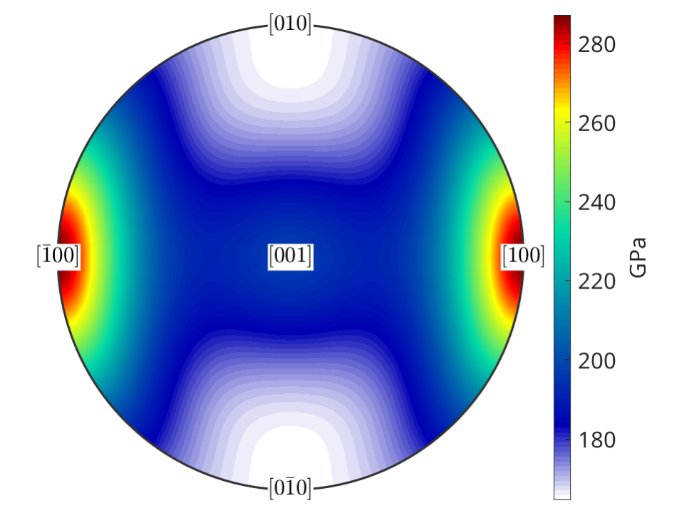
Elastic anisotropy

Code

plot(C.YoungsModulus,'complete','upper')
mtexColorbar('title','GPa')

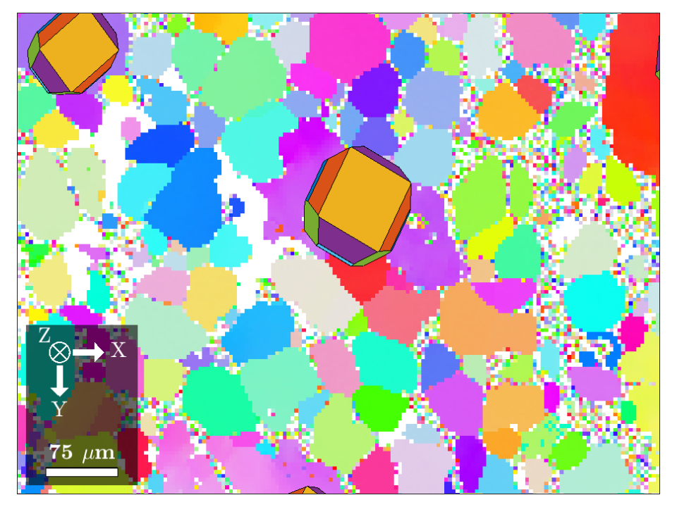
Reference frames

Code

ebsd = EBSD.load(fullfile(mtexEBSDPath,'olivineopticalmap.ang'),'setting',2);
grains = calcGrains(ebsd);
plot(ebsd('olivine'),'ipfDirection',zvector,'refFrame','on')
hold on, plot(grains(grains.numPixel>500),crystalShape.olivine,'colored'), hold off

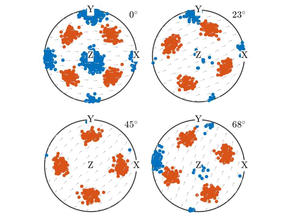
Clustering

Code

cs = crystalSymmetry('432');
odf = 0.7*fibreODF(fibre.gamma(cs),'halfwidth',10*degree) + ...
  0.3*unimodalODF(orientation.byEuler(30*degree,10*degree,60*degree,cs));
ori = odf.discreteSample(10000);
[cId,center] = calcCluster(ori,'method','classix');
plotSection(ori,ind2color(cId),'markerSize',5,'sigma','sections',4)

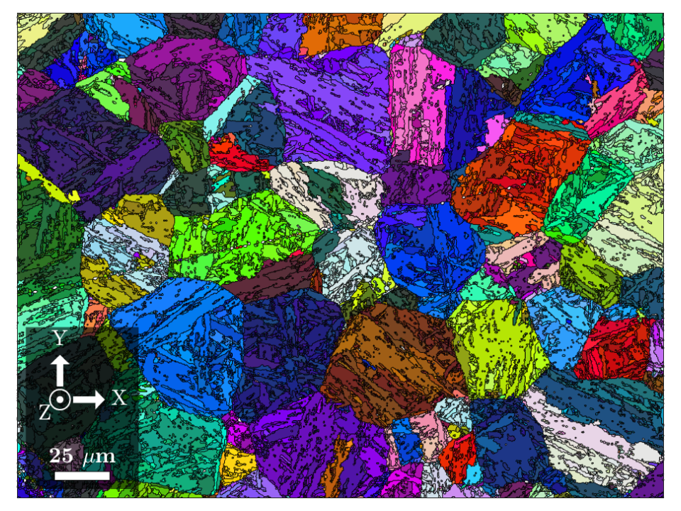
Martensite reconstruction

Code

mtexdata martensite
job = parentGrainReconstructor(ebsd);
job.p2c = orientation.KurdjumovSachs(job.csParent,job.csChild);
job.calcParent2Child;
job.calcGraph('threshold',2.5*degree,'tolerance',2.5*degree);
job.clusterGraph;
job.calcParentFromGraph;
plot(job.parentGrains,'ipfDirection',zvector)

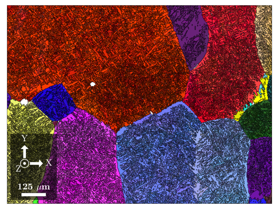
Parent grain reconstruction

Code

mtexdata alphaBetaTitanium
job = parentGrainReconstructor(ebsd);
job.p2c = orientation.Burgers(job.csParent,job.csChild);
job.calcVariantGraph('threshold',1.5*degree);
job.clusterVariantGraph('numIter',3);
job.calcParentFromVote;
plot(job.parentGrains,'ipfDirection',zvector)

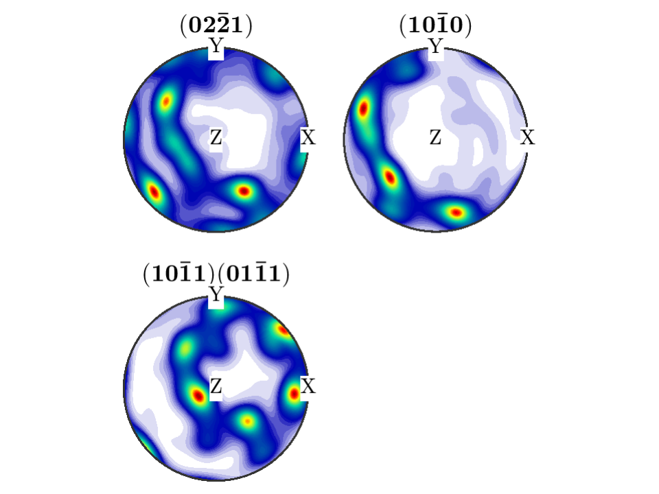
ODF reconstruction

Code

mtexdata dubna
odf = calcODF(pf,'silent');
plotPDF(odf,pf.allH(1:3),'antipodal','superposition',pf.c(1:3),'layout',[2 2])

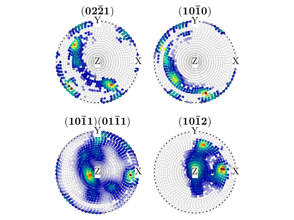
Pole figure data

Code

mtexdata dubna silent
plot(pf{1:4},'layout',[2 2],'markerSize',4)

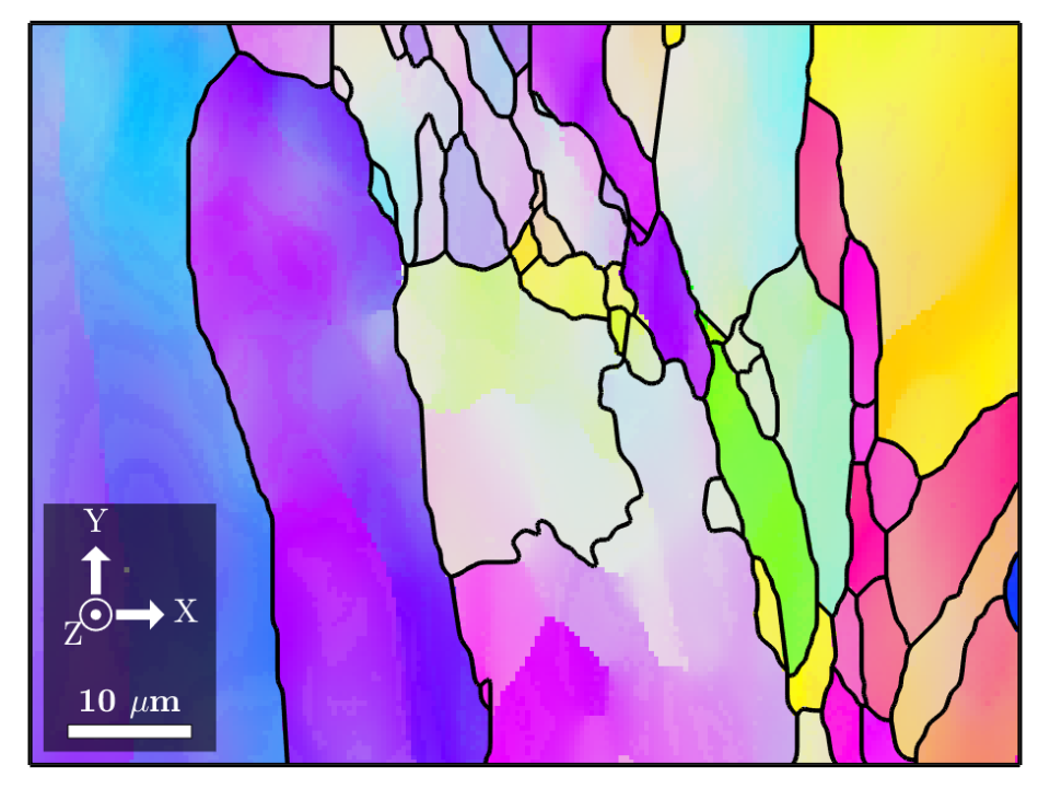
Reconstructing grains

Code

mtexdata EMSphinx silent
ebsd = ebsd('Iron fcc');
ebsd = ebsd(inpolygon(ebsd,[40 30 80 60]));
grains = calcGrains(ebsd,'fmc',0.5,'minPixel',10);
grains = smoothBoundary(grains,5);
plot(ebsd,ebsd.orientations,'ipfDirection',zvector)
hold on, plot(grains.boundary,'lineWidth',2), hold off

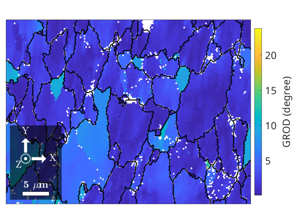
Orientation gradients within grains

Code

mtexdata ferrite silent
[grains,ebsd] = calcGrains(ebsd,'angle',10*degree,'minPixel',5);
grod = calcGROD(ebsd,grains);
plot(ebsd,grod.angle./degree)
mtexColorMap parula
mtexColorbar('title','GROD (degree)')
hold on, plot(grains.boundary,'lineWidth',1.5), hold off

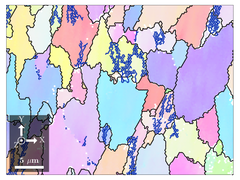
Revealing subgrain boundaries

Code

[grains,ebsd] = calcGrains(ebsd,'angle',[10 1]*degree,'minPixel',5);
subGB = grains.innerBoundary;
subGB = subGB(subGB.misorientation.angle<=10*degree & subGB.componentSize>50);
plot(ebsd('indexed'),ebsd('indexed').orientations,'faceAlpha',0.4)
hold on
plot(grains.boundary,'lineWidth',1.5)
plot(subGB,'lineWidth',2,'lineColor',[0.05 0.2 0.7])
hold off

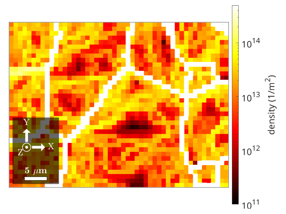
Mapping dislocation density

Code

ebsd = EBSD.load(fullfile(mtexEBSDPath,'DC06_2uniax.ang'),'setting',2);
ebsd = ebsd(inpolygon(ebsd,[1 25 48 36]));
[grains,ebsd] = calcGrains(ebsd,'angle',2.5*degree,'minPixel',6);
ebsd = smooth(ebsd,l1TVFilter,'fill',grains);
dS = dislocationSystem.bcc(ebsd.CS);
dS(dS.isEdge).u = 1;
dS(dS.isScrew).u = 0.7;
gnd = calcGND(ebsd,dS);
plot(ebsd,gnd)
mtexColorMap hot
set(gca,'ColorScale','log','CLim',[1e11 5e14]);
mtexColorbar('title','density (1/m^2)')
hold on, plot(grains.boundary,'lineWidth',1.5,'lineColor','w'), hold off

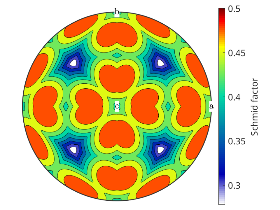
Schmid factors and slip systems

Code

cs = crystalSymmetry('432');
sS = slipSystem.fcc(cs).symmetrise('antipodal');
SF = sS.SchmidFactor;
contourf(max(abs(SF),[],1),'upper')
mtexColorbar('title','Schmid factor')

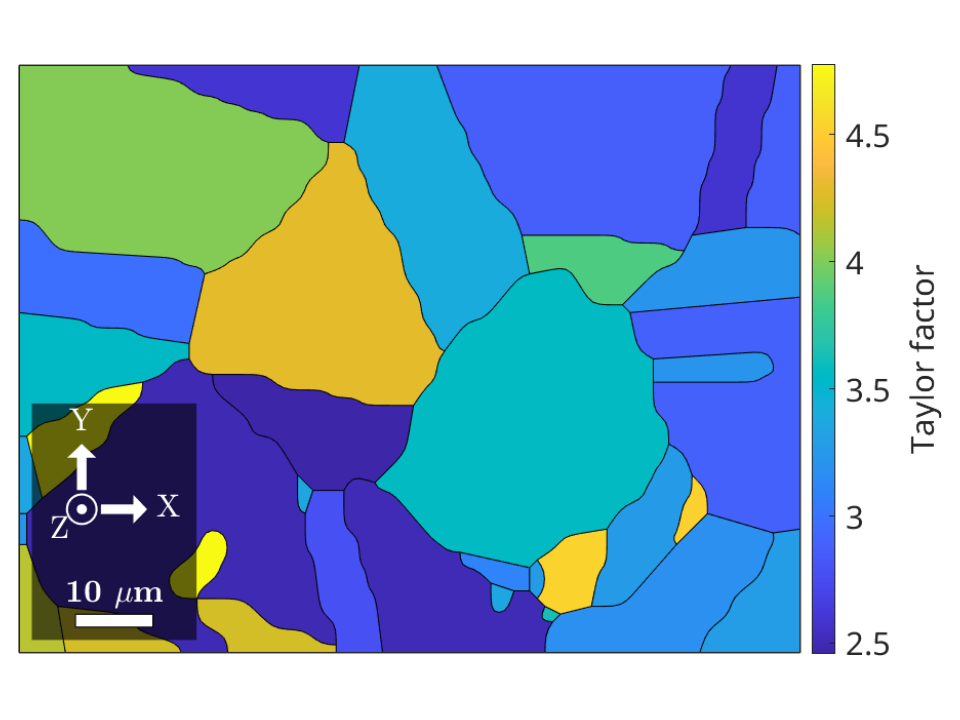
Predicting plastic deformation

Code

mtexdata csl silent
ebsd = ebsd(inpolygon(ebsd,[40 20 100 75]));
grains = smoothBoundary(calcGrains(ebsd,'minPixel',3),5);
sS = slipSystem.fcc(grains.CS).symmetrise;
epsilon = strainTensor(diag([1 0 -1]));
M = calcTaylor(inv(grains.meanOrientation)*epsilon,sS);
plot(grains,M)
mtexColorMap parula
mtexColorbar('title','Taylor factor')

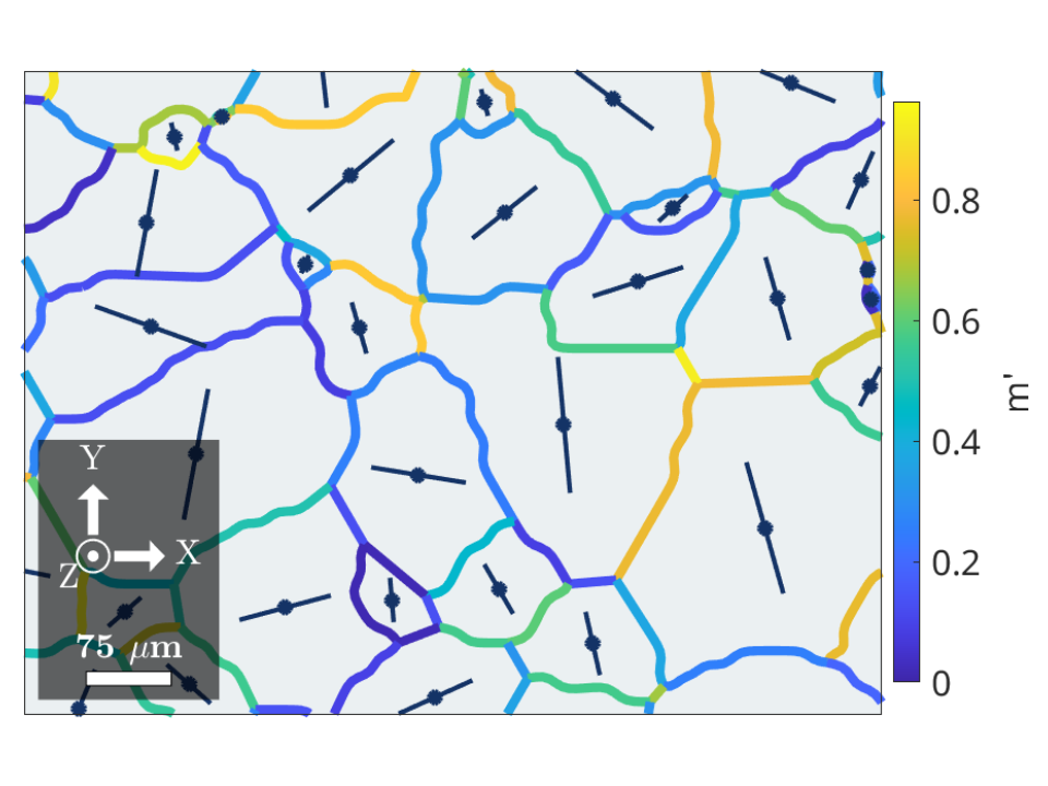
Slip across grain boundaries

Code

mtexdata titanium silent
[grains,ebsd] = calcGrains(ebsd);
grains = smoothBoundary(grains,5);
sS = slipSystem.basal(ebsd.CS).symmetrise;
[SF,id] = max(sS.SchmidFactor(inv(grains.meanOrientation)*xvector),[],2);
sSGrain = grains.meanOrientation .* sS(id);
gB = grains.boundary('indexed');
mP = mPrime(sSGrain(gB.grainId(:,1)),sSGrain(gB.grainId(:,2)));
plot(grains,'faceColor',[0.92 0.94 0.95])
hold on
plot(gB,mP,'lineWidth',4)
quiver(grains,sSGrain.trace,'color',[0.08 0.2 0.4])
hold off
mtexColorbar('title',"m'")

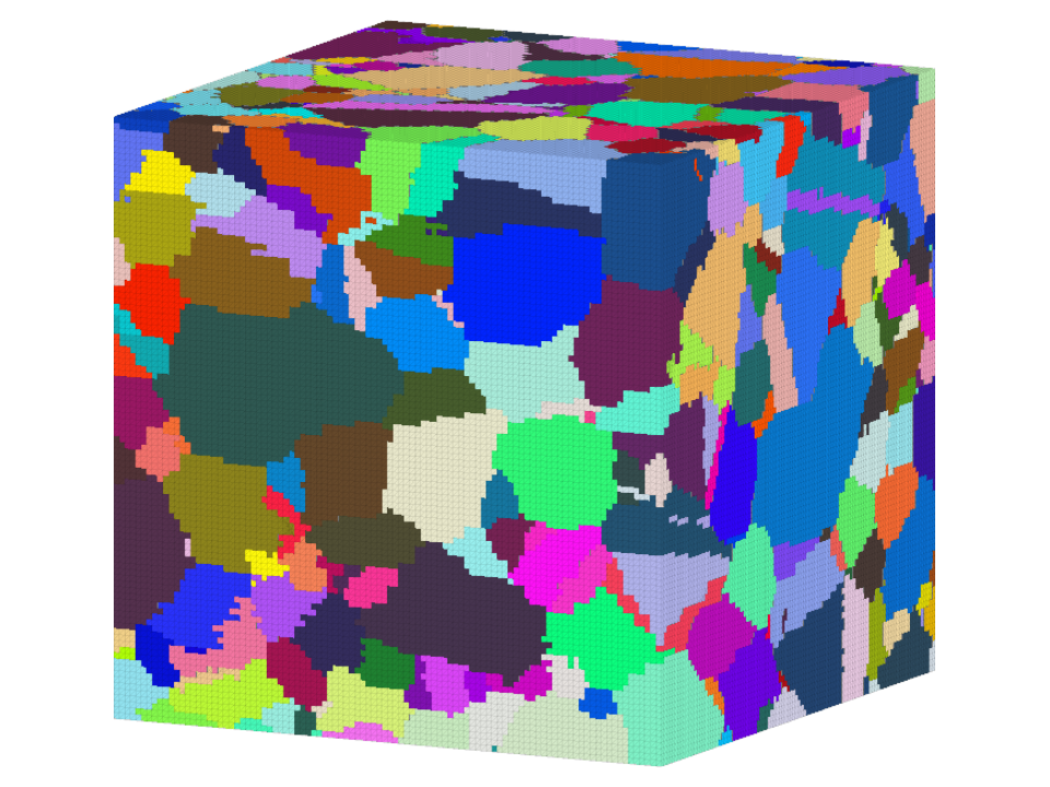
Exploring grains in 3D

Code

grains3 = grain3d.load(fullfile(mtexEBSDPath,'SmallIN100_MeshStats.dream3d'));
plot(grains3,grains3.meanOrientation,'edgeAlpha',0.08,'micronbar','off')
setCamera(plottingConvention.default3D)

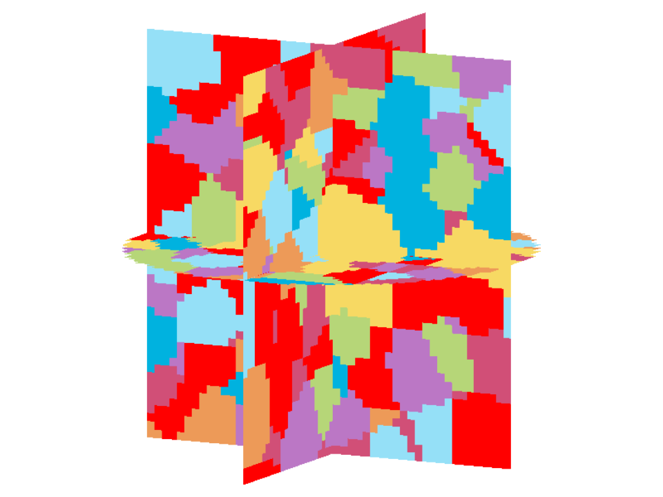
Slicing a 3D microstructure

Code

ebsd3 = mtexdata('xnovo');
plot(slice(ebsd3,plane3d(zvector,vector3d(0,0,0))),'micronbar','off')
hold on
plot(slice(ebsd3,plane3d(xvector,vector3d(0,0,0))),'micronbar','off')
plot(slice(ebsd3,plane3d(yvector,vector3d(0,0,0))),'micronbar','off')
hold off
setCamera(plottingConvention.default3D)

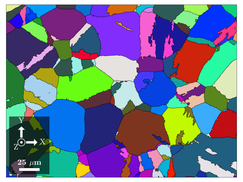
Reconstructing parent austenite

Code

mtexdata martensite silent
job = parentGrainReconstructor(ebsd);
job.p2c = orientation.KurdjumovSachs(job.csParent,job.csChild);
job.calcParent2Child;
job.calcVariantGraph('threshold',3.5*degree,'tolerance',3.5*degree);
job.clusterVariantGraph('includeSimilar');
job.calcParentFromVote;
job.mergeSimilar('threshold',7.5*degree);
job.mergeInclusions('maxSize',50);
plot(job.parentGrains,job.parentGrains.meanOrientation)

Correlating EBSD and SEM images

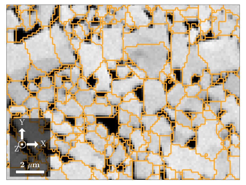
Code

mtexdata trueEbsdWCCoSmall silent
img = ebsd.opt.trueEbsdImgs;
sem = mapImage(img.fsdT1,'dxy',img.pixSzImg,'origin',ebsd.pos(1,1));
ebsd.prop.fsd = interp(sem,ebsd.pos);
plot(ebsd,ebsd.fsd)
mtexColorMap gray
hold on
grains = calcGrains(ebsd);
plot(grains.boundary,'lineColor',[1 0.65 0.1],'lineWidth',2)
hold off

Estimating texture from EBSD

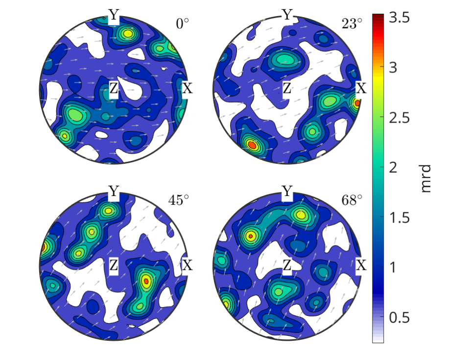
Code

mtexdata copper silent
ori = ebsd('copper').orientations;
odf = calcDensity(ori,'halfwidth',10*degree);
plotSection(odf,'sigma','sections',4,'contourf')
mtexColorbar('title','mrd')

Properties of textured polycrystals

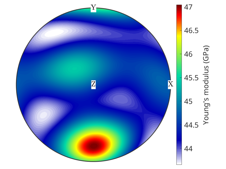
Code

mtexdata twins silent
Cij = [59.7 26.2 21.7 0 0 0;26.2 59.7 21.7 0 0 0;21.7 21.7 61.7 0 0 0;...
  0 0 0 16.4 0 0;0 0 0 0 16.4 0;0 0 0 0 0 16.75];
C = stiffnessTensor(Cij,ebsd('Magnesium').CS);
[~,~,CHill] = calcTensor(ebsd('Magnesium'),C);
plot(CHill.YoungsModulus,'complete','upper')
mtexColorbar('title',"Young's modulus (GPa)")

Understanding misorientations

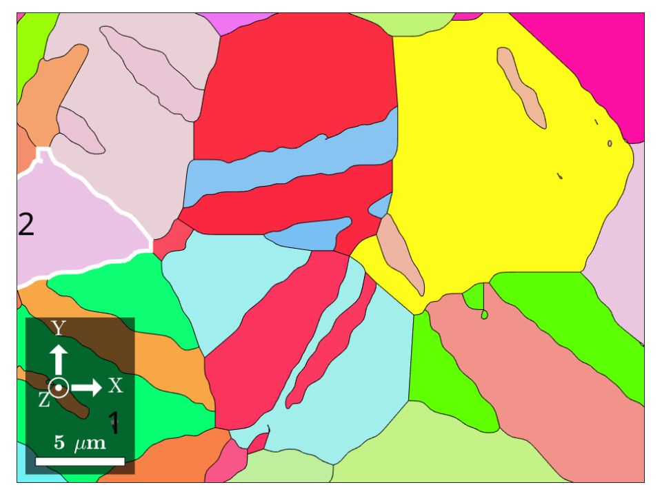
Code

mtexdata twins silent
grains = smoothBoundary(calcGrains(ebsd,'angle',5*degree),5);
plot(grains,grains.meanOrientation,'ipfDirection',zvector)
hold on
plot(grains([57 58]).boundary,'lineColor','w','lineWidth',3)
text(grains([57 58]),{'1','2'},'fontSize',22)
hold off

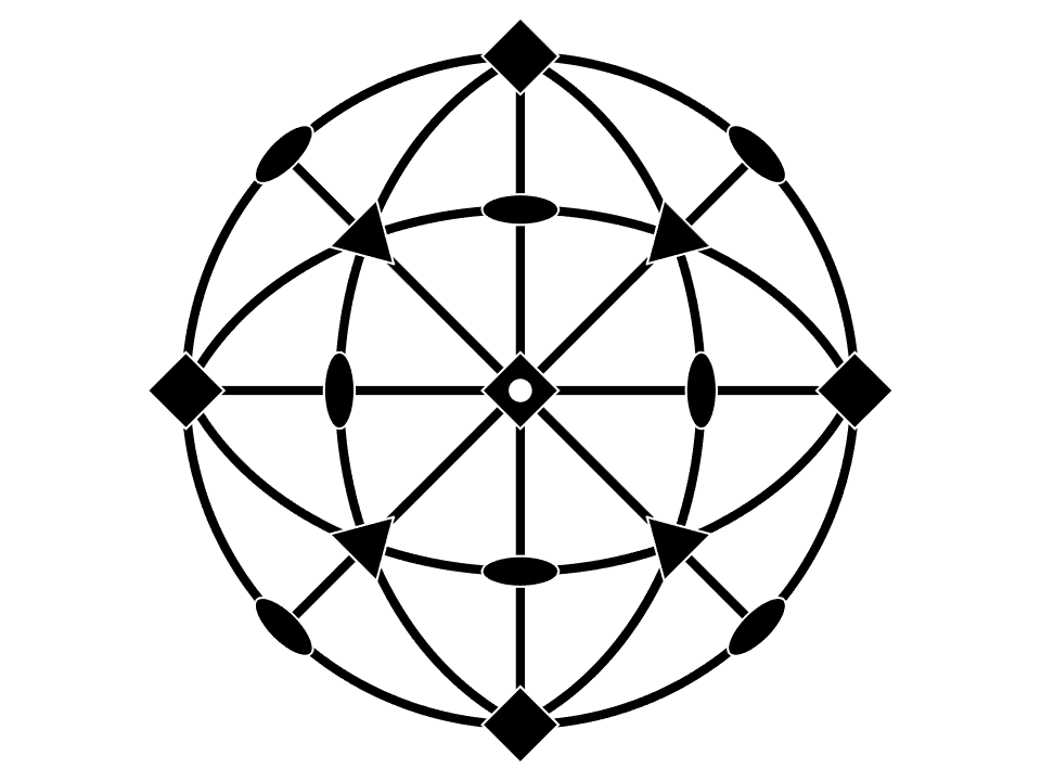
Crystal symmetry

Code

plot(crystalSymmetry('m-3m'))

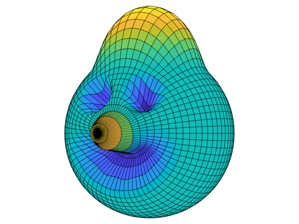
Functions on the sphere

Code

surf(S2Fun.smiley)
axis off
how2plot = plottingConvention;
how2plot.north = yvector;
how2plot.outOfScreen = vector3d(1,0,2);
setCamera(how2plot)

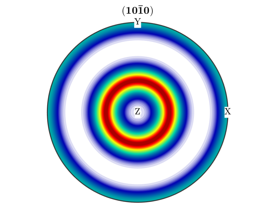
Choosing your plot style

Code

cs = crystalSymmetry('-3m');
odf = fibreODF(Miller(1,1,0,cs),zvector);
plotPDF(odf,Miller(1,0,0,cs),'antipodal')

What MTEX can do