EBSD Maps and SEM Images edit page

An EBSD map and a forescatter or backscattered-electron (BSE) image can record the same area of a specimen. Each is a raster: a rectangular array whose entries sample that area.

Comparing the two requires two independent questions to be answered:

where on the specimen each raster sits - its reference frame
which specimen direction each array index follows - its layout

A reference frame is the coordinate system in which data are expressed. Its identity, basis and plotting convention say what the axes mean and how they are drawn. A layout instead says what img(i,j) means: the direction in which the row index i and column index j increase.

Read Gridded EBSD Data first if matrix-shaped EBSD data is new to you. Reference Frame Alignment explains how map coordinates and Euler angles are related.

This page uses an EBSD map and four forescatter images of the same 20 × 15 micron WC-Co area. It first reconciles their frames, then their layouts, and finally their pixel grids.

plottingConvention.default('y↓→x');

mtexdata trueEbsdWCCoSmall silent

img = ebsd.opt.trueEbsdImgs;

Put the Map and Images in One Sequence

A mapImage combines a raster with the geometry that locates it. The geometry consists of the centre position of pixel (1,1), one step vector for each array dimension and a reference frame.

Passing an EBSD map supplies that geometry from the map. A plain image has only its pixel size here. MTEX initially gives it an independent frame. The map channel and the SEM images then form one mapImage array rather than two different container types.

imgList = [mapImage(ebsd.bc,ebsd,         'name','bcImg'), ...
  mapImage(img.fsdT1, 'dxy',img.pixSzImg, 'name','fsdT1'), ...
  mapImage(img.fsdT10,'dxy',img.pixSzImg, 'name','fsdT10')]

imgList = mapImage (y↓→x)
 
        image    pixel   frame    layout    name                 EBSD
 1   96 × 128  0.16 um    y↓→x  row↓→col   bcImg  W C, Co-fcc, Co-hcp
 2  192 × 256  0.08 um  iY↓→iX  row↓→col   fsdT1                    -
 3  192 × 256  0.08 um  iY↓→iX  row↓→col  fsdT10                    -

The table reports image size, pixel size, frame and layout for every entry. The EBSD band-contrast channel is coarser than the two forescatter images, but all three initially have the same screen alignment.

plot(imgList,'layout',[1,3],'refFrame','on')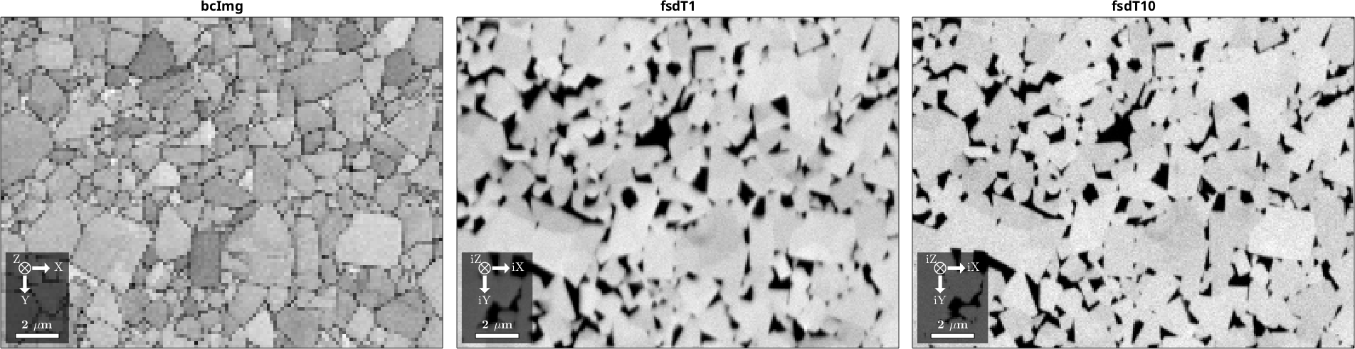

The same grain outlines appear upright and in the same part of all three panels. Their grey values need not match because the three imaging signals measure different contrast.

What an Image Does Not Know

The map entry brings the map's specimen frame with it. Its display names the specimen axes and states their screen directions.

imgList(1).frame

ans = specimenFrame (specimen, y↓→x)

A plain image array cannot reveal which specimen direction its horizontal axis follows. Until that relation is supplied, MTEX uses a separate frame. Its axes iX, iY and iZ expose rather than hide that independence.

imgList(2).frame

ans = specimenFrame (image, iY↓→iX)

Two Pictures That Disagree

The original data were collected in one session, so the images above agree. To construct the other case, rotate the EBSD map through 90 degrees. This represents a stage rotation between the map and image acquisitions.

ebsd = rotate(ebsd,90*degree);

imgList = [mapImage(ebsd.bc, ebsd,         'name', 'bcImg'), ...
  mapImage(img.fsdT1, 'dxy', img.pixSzImg, 'name', 'fsdT1'), ...
  mapImage(img.fsdT10,'dxy', img.pixSzImg, 'name', 'fsdT10')]

imgList = mapImage (y↓→x)
 
        image    pixel   frame    layout    name                 EBSD
 1   128 × 96  0.16 um    y↓→x  row↓→col   bcImg  W C, Co-fcc, Co-hcp
 2  192 × 256  0.08 um  iY↓→iX  row↓→col   fsdT1                    -
 3  192 × 256  0.08 um  iY↓→iX  row↓→col  fsdT10                    -

The map is now a 128 × 96 array, whereas each image is 192 × 256. Their long and short dimensions are interchanged. Only the size column changed: the rotation moved the data, not the recorded convention, so both frame columns still read down-then-right and the table gives no sign that the three rasters have fallen out of step.

plot(imgList,'layout',[1,3],'refFrame','on')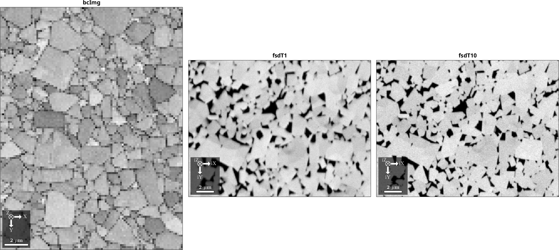

The pictures show what the table does not. The EBSD panel now stands upright beside two landscape images and occupies a different specimen extent, while the frame indicators in the corners still read the same arrangement in all three panels.

Establish the Frame Relation on Screen

A plotting convention states how a reference frame is laid out on screen. It never changes the data. Set the map frame so that its x axis points up and its y axis points right. The image frames keep their original setting.

This alignment is experimental information. No inspection of the array values can recover it. Use acquisition metadata or a known specimen feature.

ebsdFrame = imgList(1).frame;
ebsdFrame.how2plot = 'x↑→y';

plot(imgList,'layout',[1,3])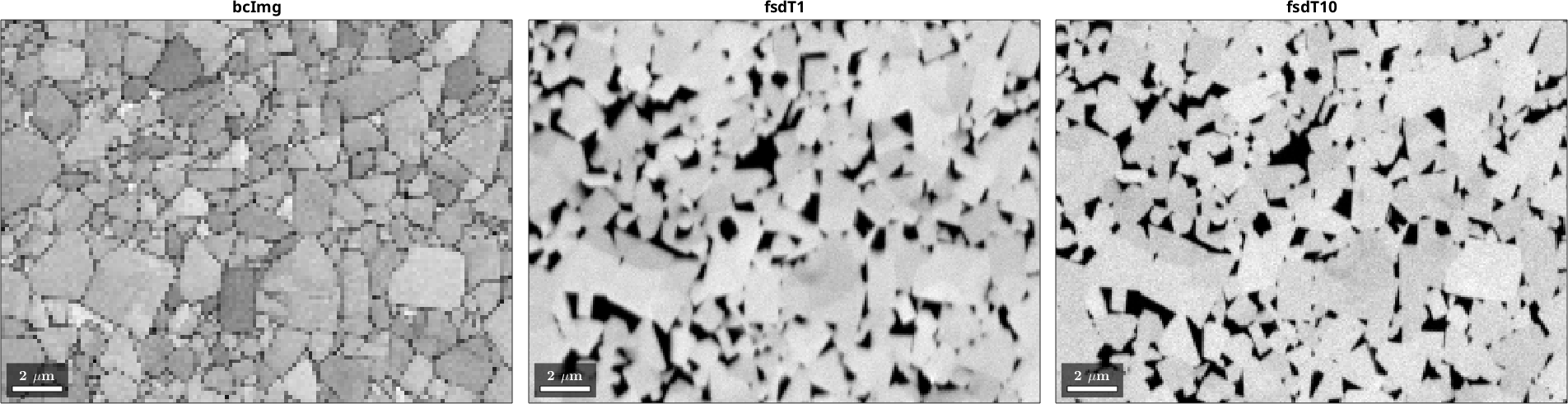

The corresponding grain outlines are now the same way up. Changing how2plot only established how the two frames appear on screen. It has not yet expressed the images in the map frame.

byScreenAlignment records the assertion that the plotted frames are physically aligned. transformReferenceFrame then re-expresses every entry in the map frame.

imgList = transformReferenceFrame(imgList,ebsdFrame,'byScreenAlignment')

imgList = mapImage (x↑→y)
 
        image    pixel  frame    layout    name                 EBSD
 1   96 × 128  0.16 um   x↑→y  row↓→col   bcImg  W C, Co-fcc, Co-hcp
 2  192 × 256  0.08 um   x↑→y  row↓→col   fsdT1                    -
 3  192 × 256  0.08 um   x↑→y  row↓→col  fsdT10                    -

The new table shows one common frame and the corresponding layouts. This operation only transposes or flips the arrays and updates their geometry; it does not resample any values.

plot(imgList,'layout',[1,3])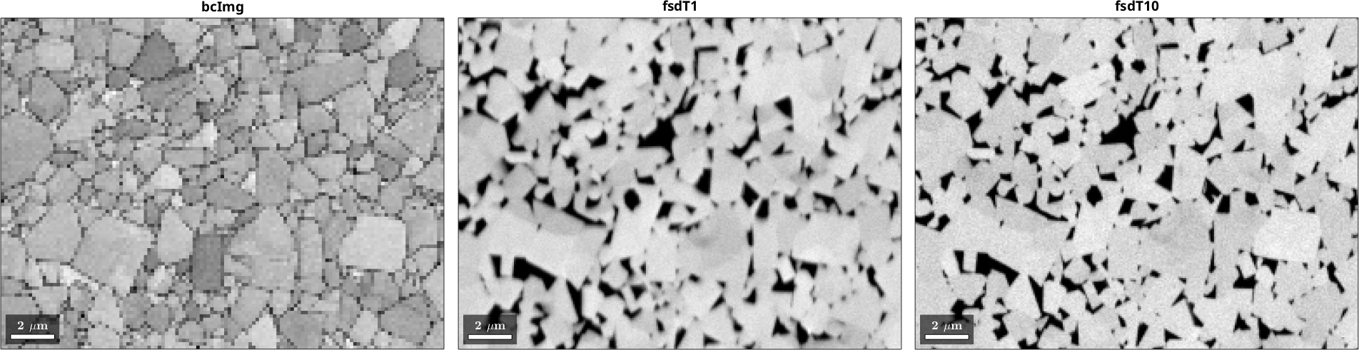

The panels remain the same way up after the frame change. That unchanged appearance is the point. The arrays and their frame labels changed together, while the physical pictures did not.

How the Array Is Stored

The transformed table also shows that the map changed from 128 × 96 back to 96 × 128. This is the second question, and it is independent of the specimen frame.

A gridLayout contains two directions. The first is the direction in which the row index advances, and the second is the direction in which the column index advances.

imgList(1).layout

ans = gridLayout (row||-x, col||y)

Every mapImage states its layout, and so does every gridded EBSD map.

ebsd.layout

ans = gridLayout (row||y, col||x)

Put a Map in an Image Layout

gridify accepts a layout and stores a square-grid map in that order. Gridded EBSD Data introduces the named layouts 'columnMajor' and 'rowMajor'. Give any other signed pair of axis directions as a gridLayout.

Start again from the imported map. Suppose the detector was mounted a quarter turn from the scan. Its rows run against x and its columns along y.

mtexdata trueEbsdWCCoSmall silent

gL = gridLayout(-xvector,yvector)

gL = gridLayout (row||-x, col||y)

Store the map in that layout and display its resulting matrix shape.

ebsdI = gridify(ebsd,gL);

size(ebsdI)

ans =
   128    96

No measurement was resampled or invented. On the same square lattice, a layout change applies only a transpose and two possible flips. It is safe for orientation data. For this pair the result is exactly a quarter turn.

isequal(ebsdI.bc,rot90(ebsd.bc))

ans =
  logical
   1

Returning to the original layout is exact as well.

isequal(gridify(ebsdI,ebsd.layout).bc,ebsd.bc)

ans =
  logical
   1

The specimen has not moved. A layout changes how measurements are stored, not where they are. MTEX adjusts the screen mapping, so both maps still plot the same way up.

plot(ebsd,ebsd.bc,'micronbar','off','layout',[1,2]), mtexColorMap gray
title('as imported')
nextAxis
plot(ebsdI,ebsdI.bc,'micronbar','off'), mtexColorMap gray
title('row ||-x, col ||y')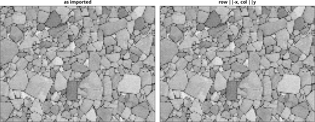

The same WC grains occupy the same screen positions in both panels even though the two band-contrast matrices are quarter-turn permutations.

Compare the Rasters Pixel by Pixel

Agreeing frames and layouts makes the rasters geometrically comparable, but pixel-wise operations also require one common grid. The EBSD spacing is 0.159 micron here, whereas the image spacing is 0.0795 micron.

interp samples an image at arbitrary positions. A bare array carries no physical origin, so state where the centre of its first pixel lies. The origin and pixel size must use the same length unit as the EBSD positions.

mgI = mapImage(img.fsdT1,'dxy',img.pixSzImg,'origin',ebsd.pos(1,1));

ebsd.prop.fsdT1 = interp(mgI,ebsd.pos);

The image is now a per-pixel property: one value per measurement point, indexed and subset in lockstep with the map. It travels through cropping, gridding and indexing with the EBSD data. The two channels can now be passed side by side to image-processing tools.

Image values are interpolated linearly by default, and positions outside the image return NaN. No EBSD orientation is interpolated in this step.

plot(ebsd,ebsd.bc,'micronbar','off','layout',[1,2])
title('band contrast')
nextAxis
plot(ebsd,ebsd.fsdT1,'micronbar','off')
title('forescatter on EBSD grid')
mtexColorMap gray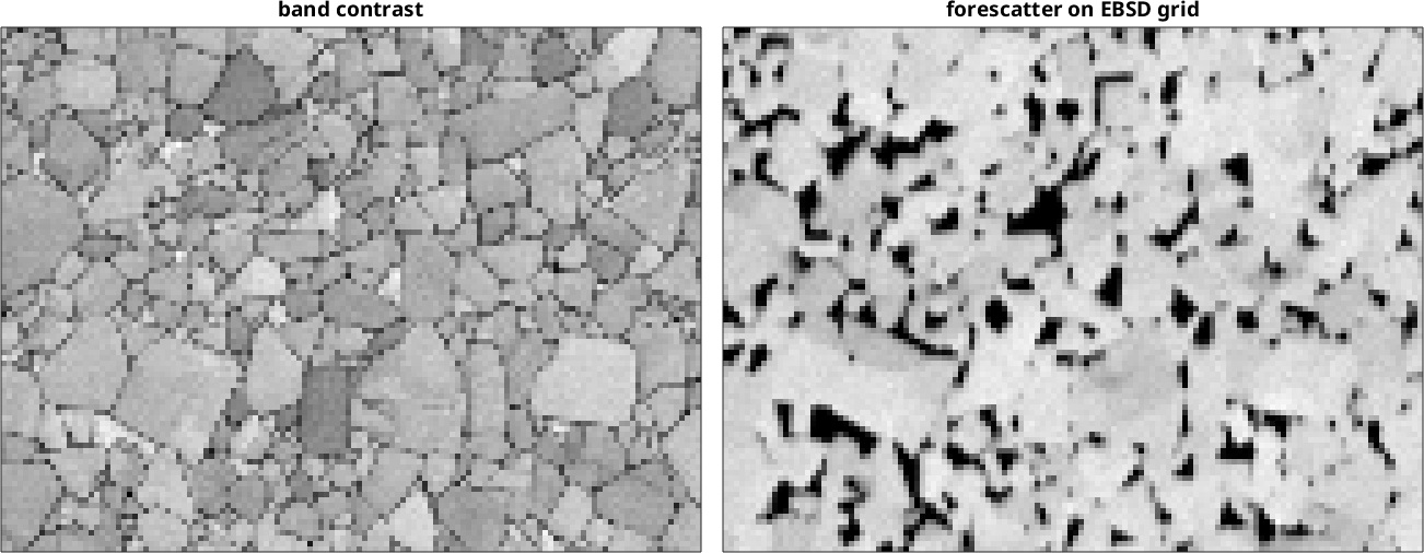

The same grain-scale features occupy roughly the same places in both panels. Their edges do not overlay perfectly, which shows that matching frames, layouts, origins and pixel sizes is necessary but not sufficient.

From Bookkeeping to Registration

Beam drift during a scan, camera motion between acquisitions and specimen tilt all change positions continuously. They are not layout problems. Each is a spatial transform that can be fitted from corresponding image features and then removed.

TrueEBSD Distortion Correction performs that workflow. It starts with exactly the sequence built here: entries that agree about the specimen frame, array order and pixel grid.

EBSD Maps and SEM Images