TrueEBSD Distortion Correction

An EBSD map and an SEM image of the same area never quite line up: the beam drifts during the scan, the camera moves between acquisitions, the specimen is tilted. TrueEBSD corrects that, so every pixel of the map and every pixel of the images refers to the same point on the specimen. What comes out is an ordinary EBSD map that carries the images as per-pixel properties.

TrueEBSD was first published as a separate toolbox by Vivian Tong and Stefan Olovsjö of Seco Tools AB, R&D Materials and Technology, Fagersta, Sweden. Tong et al. describe its MTEX implementation and correlative applications in arXiv 2605.00703.

This page runs the whole workflow on a cut-down WC-Co dataset in well under a minute. First read Maps and Images to prepare a common specimen frame, array layout and length unit. See Spatial Transforms for choosing a distortion model, trueEbsd for the workflow class and mapImage for its image container.

TrueEBSD corrects map positions. It does not repair an incorrect relation between Euler angles and the specimen frame, and it does not correct an orientation error caused during acquisition. Use Reference Frame Alignment for the first problem.

The convention set here only decides which way up the figures come out. It has no effect on the correction: a map entry's array order is read off its own d1 and d2, and no plotting convention is consulted anywhere in the workflow.

plottingConvention.default('y↓→x');

mtexdata trueEbsdWCCoSmall silent

display(ebsd.opt.trueEbsdImgs)

struct with fields:

       fsdB3: [192×256×3 double]
       fsdT3: [192×256 double]
       fsdT1: [192×256 double]
      fsdT10: [192×256 double]
    pixSzImg: 0.0795

The structure lists four same-area SEM images and their pixel size. The EBSD map itself supplies the fifth image below through its band contrast.

Build the Sequence

TrueEBSD does not jump straight from the EBSD map to the reference image. It steps through the images one pair at a time, correcting one kind of distortion at each step - which is why there are four images rather than one. Each pair differs by something simple enough to model, whereas the map and the final image differ by everything at once.

The order therefore matters. It runs from the most distorted map to the ground-truth reference. The images go in one list and the distortions in another, one per hop. The last image is the fixed reference and does not move.

'name' is what each image is called once it is attached to the map at the end, so the result reads as ebsdOut.fsdT1.

img = ebsd.opt.trueEbsdImgs;

imgList = [mapImage(ebsd.bc, ebsd,                  'name','bcImg'), ...
  mapImage(img.fsdB3,  'dxy',img.pixSzImg, 'name','fsdB3'), ...
  mapImage(img.fsdT3,  'dxy',img.pixSzImg, 'name','fsdT3'), ...
  mapImage(img.fsdT1,  'dxy',img.pixSzImg, 'name','fsdT1'), ...
  mapImage(img.fsdT10, 'dxy',img.pixSzImg, 'name','fsdT10')];

A light box filter first - cross-correlation dislikes noise - and one common range, since the levels off different detectors mean nothing to each other. Both are methods of mapImage and both take the whole list at once.

imgList(2:end) = rescale(imboxfilt(imgList(2:end),3));

The distortions are objects, one per hop, not names on the images: beam drift plus a rigid offset, then nothing, then the camera moving, then the specimen tilt seen at a different kV. There are five maps and so four hops, and the reference has no entry of its own - where nothing separates a pair that is spatialTransformId.

A multi-stage model is built with + and not *. + reads left to right in the order the stages are applied and keeps both of them, where an unfitted prototype has zero coefficients, so it reports itself as the identity and * would absorb it away.

T = [spatialTransformShift + spatialTransformDrift, ...
  spatialTransformId, ...
  spatialTransformShift, ...
  spatialTransformTilt];

The job holds the whole workflow, and each step below adds to it. Building it also checks that the sequence really is stored one consistent way round, and that every entry measures the sample in the same unit.

job = trueEbsd(imgList,T)

job = trueEbsd (as imported)
 
      name          image   distortion  shift, px  residual, px
 1   bcImg       96 × 128  shift-drift          -             -
 2   fsdB3  192 × 256 × 3     identity          -             -
 3   fsdT3      192 × 256        shift          -             -
 4   fsdT1      192 × 256         tilt          -             -
 5  fsdT10      192 × 256                       -             -

Plot the sequence to check the images really do cover the same area. Note how different the contrasts look - that is why matching is done on edges rather than on the original values.

plot(imgList)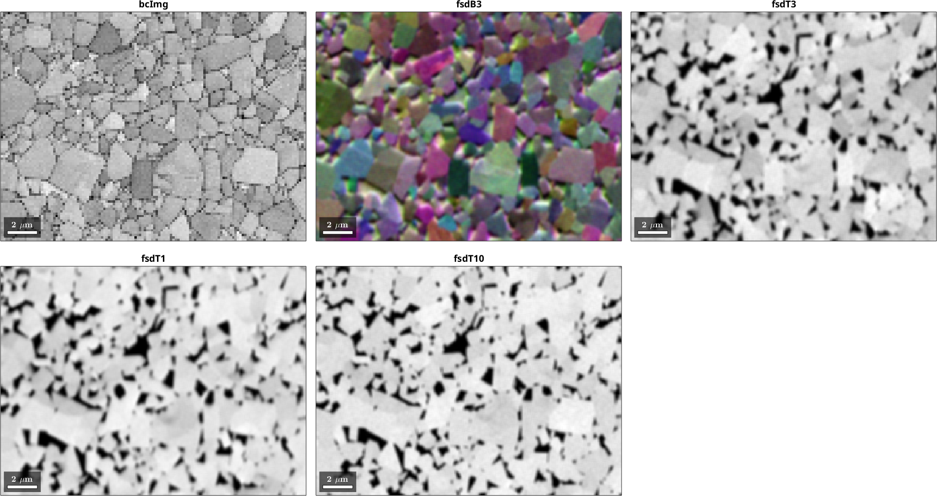

The same WC grain network is visible in every panel, but its edges do not yet occupy the same positions. Each hop displaces the map in its own direction, and those directions partly cancel along the chain: the shifts fitted below come to about (3.9, 5.5) pixels for the first hop and (-2.8, -1.9) for the third, which leaves the last panel closer to the first than the first two panels are to each other.

Put Everything on One Pixel Grid

The map is on a 0.159 µm grid and the images on 0.0795 µm. pixelSizeMatch resamples them all onto the finest one, so pixel (i,j) means roughly the same place in each. Give it a pixel size to ask for a particular grid; with no argument it takes the smallest present.

Images are interpolated linearly. EBSD data is not: orientations and phase labels have no meaningful average, so the nearest measured point is used.

Nothing has been corrected yet - this is only bookkeeping.

job.pixelSizeMatch;

using default pixel size of 0.079501 um, minimum from imgList

The resampled sequence is in job.resizedList.

display(job.resizedList,'variableName','job.resizedList')

job.resizedList = mapImage (y↓→x)
 
            image    pixel   frame    layout    name                 EBSD
 1      192 × 256  0.08 um    y↓→x  row↓→col   bcImg  W C, Co-fcc, Co-hcp
 2  192 × 256 × 3  0.08 um  iY↓→iX  row↓→col   fsdB3                    -
 3      192 × 256  0.08 um  iY↓→iX  row↓→col   fsdT3                    -
 4      192 × 256  0.08 um  iY↓→iX  row↓→col   fsdT1                    -
 5      192 × 256  0.08 um  iY↓→iX  row↓→col  fsdT10                    -

Adjust the Matching Windows

Distortions are measured by cutting both images of a pair into small boxes and cross-correlating each box with its partner - see xcfShift. That gives a local shift at each box, and those shifts are fitted to the distortion model.

Almost none of it has to be specified. The box width roiSize and the edgeWidth below are measured from the images themselves the first time calcDistortion needs them, and what was chosen is printed so it can be overridden. Both are lengths, in the map's own scanUnit, so they mean the same thing before and after pixelSizeMatch and may be set at any point.

What is worth setting here is how many boxes to use. The default of 24 across suits a full-size map; this grid is small, and the matching is the entire runtime, so fewer is quicker.

job.setOptions('numROI',16);

Measure the Distortion

These are the pictures that will actually be matched. A band contrast map and a backscatter image have nothing in common as grey values, but their grain boundaries fall in the same places - which is why the edge transform is what gets correlated, and why registerOn defaults to 'edge'. Set it to 'raw' for a pair that already shares contrast.

plot(job.resizedList,'edge')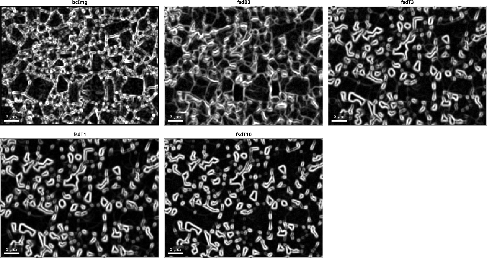

Corresponding WC boundaries now appear as bright lines in every panel. Those shared lines, rather than the detector-dependent grey levels, are what each local cross-correlation window matches.

'fitErr' re-measures the shifts after each correction and reports what is left over. That residual is how you tell whether it worked: around a pixel or less is good.

Both columns read as a length followed by the signed x and y behind it, in pixels of the common grid: how far the step moved the map, and which way. Where the length and signed components agree, the correction was one coherent movement - a specimen drift or a camera offset has a direction. Where the signed pair falls to nearly zero against a large length, the boxes disagree with each other and the correlation found no common direction.

If a residual comes out above two pixels, TrueEBSD doubles the box size and tries again, repeating until it comes down or the box outgrows the image. On the first hop here, the automatic 32 px box leaves 3.36 px and triggers one 64 px retry. The residual then falls to 1.53 px.

Steps whose transform is spatialTransformId are skipped: nothing separates that pair, so their shift is taken as zero. The displayed difference for that hop is the raw image difference, not a fitted residual and not a correction to apply.

job.calcDistortion('fitErr');

◆ measured settings, override with setOptions
   ▸ edgeWidth  per map  4 4 5 5 5 px
   ▸ roiSize    per hop  32 64 64 64 px   ← shifts 5.0 2.2 3.3 3.5 px, features 4 7 7 7 px

 ◆ distortion across 5 maps, 4 hops

    distortion   stage              ROI          shift, px       residual, px
    ──────────── ───────────── ──────── ────────────────── ──────────────────
  ● bcImg
  │ shift-drift  shift            32 px 4.19 (+0.99,+0.12)
  │              drift            32 px 3.72 (+0.33,+0.34)
  │              ↳ residual                                3.36 (+0.26,+0.19)
  │ ↻ residual over 2 px, retrying with a 64 px ROI
  │ shift-drift  shift            64 px 3.64 (+2.20,+1.84)
  │              drift            64 px 2.04 (+0.23,+0.49)
  │              ↳ residual                                1.53 (+0.07,+0.09)
  ▼
  ● fsdB3
  │ identity     ·                    · 0.00 (+0.00,+0.00)
  │              ↳ difference                              2.03 (-0.14,-1.50)
  ▼
  ● fsdT3
  │ shift        shift            64 px 3.25 (-2.69,-1.81)
  │              ↳ residual                                0.27 (+0.16,+0.15)
  ▼
  ● fsdT1
  │ tilt         projective       64 px 3.61 (+2.86,-2.19)
  │              poly11           64 px 0.27 (+0.06,-0.09)
  │              poly22           64 px 0.27 (+0.05,-0.09)
  │              ↳ residual                                0.26 (+0.06,-0.10)
  ▼
  ● fsdT10

Afterwards job.T holds the fitted transforms rather than the prototypes it started from.

display(job.T,'variableName','job.T')

job.T = spatialTransform
 size: 1 × 4
 
    model        stage       parameters                                   
 1  shift-drift  shift       scale 1.002 × 0.9614, rotate -0.0207°, shear 
                             -1.26°, move (0.175, 0.1398)                 
                 drift       10 knots over -3.617 .. 3.935, |u| <= 0.06812
 2  identity     ·           ·                                            
 3  shift        ·           scale 1.002 × 0.9998, rotate 0.048°, shear   
                             -0.0349°, move (-0.2142, -0.144)             
 4  tilt         projective  perspective (-5.27e-05, 0.000238)            
                 poly11      |c| = 0.009417                               
                 poly22      |c| = 0.01471

Correct It

Each map is now moved by the shifts of every step between it and the reference. The reference itself does not move.

Resampling is nearest-neighbour throughout, so no orientation and no phase label is ever invented by averaging two real measurements.

job.undistort;

plot(job.undistortedList)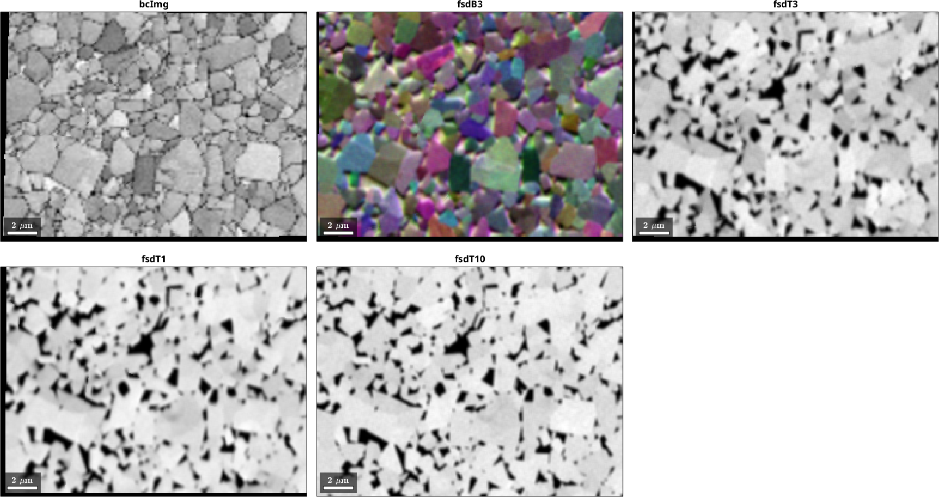

The outer rectangle was already shared: pixelSizeMatch put every entry on the same grid and the same extent. What has changed is inside it. The same WC boundaries now occupy the same positions from the band-contrast map through to the fixed reference. Small intensity differences remain because alignment does not make the detectors measure the same signal.

Use the Result

Every image is now attached to the EBSD map as a per-pixel property, under the 'name' given earlier. So ebsdOut.fsdT1 is just another map property, and plot(ebsdOut,ebsdOut.fsdT1) works like any other plot. It needs no conversion and stays with the map through cropping, gridding and indexing.

Plotting them back onto the map is also the quickest check that nothing came out the wrong way round.

fsdB3 is a colour image and keeps all three channels. Plotting onto a map needs one value per pixel, so it is averaged to grey here.

ebsdOut = job.undistortedList(1).ebsd

ebsdOut = EBSDsquare (y↓→x, row↓→col)
 
 Phase  Orientations     Mineral         Color  Symmetry  Crystal reference frame
     0   1803 (3.7%)  notIndexed          none                                   
     1   43403 (88%)         W C  LightSkyBlue      -6m2        X||a*, Y||b, Z||c
     2   3840 (7.8%)      Co-fcc  DarkSeaGreen      m-3m                         
     3   106 (0.22%)      Co-hcp     Goldenrod     6/mmm        X||a*, Y||b, Z||c
 
 Properties: bc, bs, bands, MAD, quality, oldId, bcImg, fsdB3, fsdT3, fsdT1, fsdT10
 Scan unit : um
 X × Y × Z : [-10 → 10] × [-7.6 → 7.6] × [0 → 0]
 Normal vector: (0,0,1)
 Square grid  :192 × 256
 source: trueEbsdWCCo, centre half of the field of view, coarsened 4x
 madeBy: trueEBSD tools/makeWCCoSmall.m

The summary lists bcImg, fsdB3, fsdT3, fsdT1 and fsdT10 with the other per-pixel properties. This is an ordinary EBSD map rather than a separate registration result type.

The orientation panel below is coloured by the inverse pole figure of zvector. This page draws y downwards, and that convention puts z into the screen, which the axes inset in each panel shows.

newMtexFigure('layout',[2,3],'figSize','huge');
nextAxis
plot(ebsdOut('W C'), ebsdOut('W C').orientations, ...
  'ipfDirection',zvector,'coordinates','on')
title('Undistorted EBSD map (WC IPF into screen)','Color','k')

for n = 1:numel(job.undistortedList)

  im = ebsdOut.(job.undistortedList(n).name);
  if size(im,3) > 1, im = mean(im,3); end

  nextAxis
  plot(ebsdOut, im, 'coordinates','on')
  mtexColorMap gray
  title(['Undistorted ' job.undistortedList(n).name],'Color','k')
end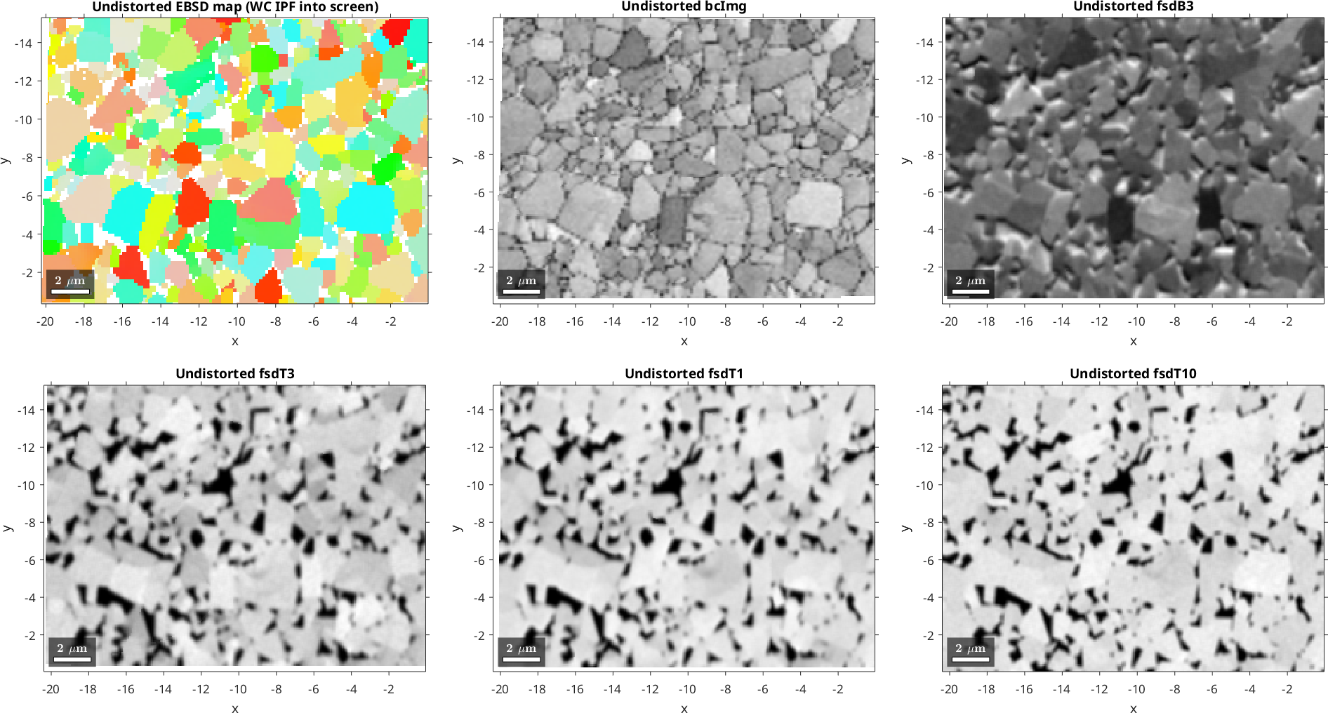

Compare the WC outlines in the orientation panel with the grey-level edges in the five image panels. The same boundaries meet the coordinate grid at the same places, which is the visual check that the arrays were neither transposed nor flipped during correction.

Finish

The map and the images now overlay pixel for pixel, and ebsdOut is an ordinary EBSD map that happens to carry four SEM images as properties. Anything you would normally do with a map works from here - including turning a thresholded image into a phase.

trueEbsdWCCoSmall is the centre half of the full WC-Co field of view coarsened by four: a 20.4 × 15.3 µm area with WC grains about 12 px across. It is small enough to be quick and still large enough for every distortion to be measurable. The full dataset is trueEbsdWCCo, and the same script runs on it unchanged - it simply takes minutes rather than seconds.

References

Next

The aligned SEM channels can now take part in normal EBSD analysis. For example, continue with grain reconstruction before measuring phase fractions, contiguity or boundary-conditioned image signals. Use Denoising only for orientation noise; denoising and spatial distortion correction solve different problems.

References

- V. S. Tong and T. B. Britton, TrueEBSD: Correcting spatial distortions in electron backscatter diffraction maps, Ultramicroscopy 221, 113130, 2021, introduces the physically staged correction and its use of intermediate images.
- V. Tong, S. Olovsjö, R. M'Saoubi, M. Grabner, M. Petersmann and L. Wright, TrueEBSD in MTEX: automatic image matching for correlative microscopy applications, arXiv:2605.00703, 2026, describes the MTEX implementation and the WC-Co application used here.
- G. Nolze, Image distortions in SEM and their influences on EBSD measurements, Ultramicroscopy 107, 172--183, 2007, relates specimen tilt and scan geometry to spatial and orientation errors.
- M. Guizar-Sicairos, S. T. Thurman and J. R. Fienup, Efficient subpixel image registration algorithms, Optics Letters 33, 156--158, 2008, gives the Fourier-domain cross-correlation method underlying the local shift measurement.