Misorientations at grain boundaries

A grain-boundary misorientation is the rotation from the crystal on one side of a boundary to the crystal on the other. It has an angle and an axis, but those two quantities answer different questions.

The angle is one number and can be drawn along the boundary directly. The axis is a direction, so its reference frame decides what it means. A crystal-frame axis can be compared with lattice directions, whereas a specimen-frame axis can be compared with directions in the map.

This page assumes that the map has already been divided into grains. See Grain Reconstruction for that step. Grain Boundary Properties introduces the segment properties used below. Misorientation Theory develops the symmetry of a misorientation.

close all;

% load the example map in its specimen plotting frame
plottingConvention.default('y↑→x');
mtexdata forsterite silent

% select a small region so that the boundary-axis arrows remain legible
region = [25000 4500 10000 4500];
ebsd = ebsd(inpolygon(ebsd,region));

Reconstruct the boundary network

A 10 degree segmentation angle separates low- from high-angle boundaries. Angles of 10 or 15 degrees are long-standing conventions, and the useful value depends on the material. Grain Reconstruction explains how to choose it. Here 'minPixel' marks indexed regions of fewer than 10 measurements as notIndexed, so that specks do not enter the boundary statistics below.

segAngle = 10*degree;
minPixel = 10;
[grains,ebsd] = calcGrains(ebsd,'angle',segAngle,'minPixel',minPixel);

% preserve the segment-to-pixel relation needed below
grains = smoothBoundary(grains,4,'noSimplify','noRefine');

% draw the forsterite grains and the complete boundary network
plot(grains('Fo'),'FaceColor',[0.75 0.82 0.90],...
  'micronbar','off','figSize','large')
hold on
plot(grains.boundary,'lineWidth',1)
hold off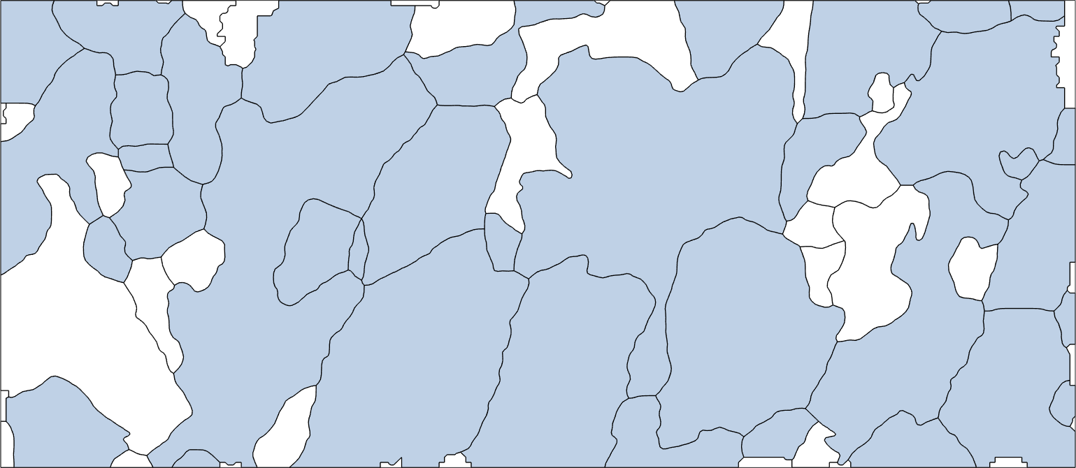

The blue regions are forsterite grains. The white regions belong to other phases, and the black lines are all boundary segments in the cropped map. The analysis below uses only boundaries between two forsterite grains.

The smoothBoundary flags 'noSimplify' and 'noRefine' are important here. Simplification and refinement change which segments lie between specific pixel pairs. Their ebsdId values can then no longer supply the two orientations used below.

The misorientation angle along a boundary

Select one phase pair before comparing misorientations. The command below also gives these same-phase misorientations grain exchange symmetry. The two grains have no intrinsic order. A rotation and its inverse therefore describe the same boundary. See Grain Exchange Symmetry.

gB = grains.boundary('Fo','Fo');

% use a neutral background so that only the boundary carries data colours
newMtexFigure('figSize','large');
plot(grains('Fo'),'FaceColor',[0.9 0.9 0.9],'micronbar','off')
hold on

% colour each segment by its angle
lineWidth = 6;
plot(gB,gB.misorientation.angle./degree,'lineWidth',lineWidth);
hold off
mtexColorMap jet
mtexColorbar('title','misorientation angle in degrees')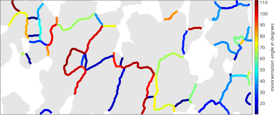

Long runs have nearly constant colour. Each segment stores the misorientation between its two neighbouring EBSD measurements. Small changes along a run reflect orientation variation inside the two grains. Larger colour changes occur between different grain pairs.

Crystal-frame and specimen-frame axes

A reference frame is the coordinate system in which data are expressed. The crystal frame is fixed to the lattice basis, while the specimen frame is fixed to the sample and supplies the coordinates of this map.

The axis of gB.misorientation is expressed in the crystal frame. This form can be compared with crystallographic directions. The stored rotation contains no specimen-frame information. Computing a specimen-frame axis requires both orientations beside every segment.

ebsdId is an \(N \times 2\) matrix of measurement IDs. It retrieves the two orientation lists without confusing persistent IDs with positions in the current EBSD list.

ori = ebsd('id',gB.ebsdId).orientations;
specimenAxes = axis(ori(:,1),ori(:,2),'antipodal');

% segments are in walk order, so regular indexing thins every chain evenly
sampleId = 1:3:length(gB);
hold on
quiver(gB(sampleId),specimenAxes(sampleId),...
  'lineWidth',2,'color','k','autoScaleFactor',0.3)
hold off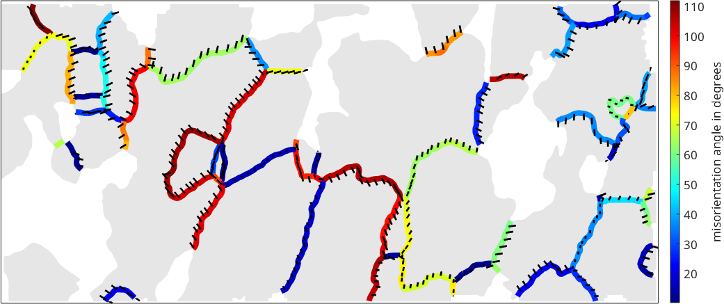

Each black line is an unoriented axis projected into the section plane. A short line marks an axis that points steeply out of the plane. The axes remain nearly parallel along most boundaries. This agrees with the nearly constant angle colours beneath them.

When the axis jumps

Along a few boundaries the projected axis changes abruptly, although the orientations within the two grains are as uniform as elsewhere. This is not necessarily a feature in the specimen. It can be a change in which symmetry-equivalent rotation MTEX selects.

Crystal symmetry gives many rotations that describe the same physical relationship. The representative with the smallest angle is the disorientation. Near a boundary of the misorientation fundamental region, two representatives can have almost the same angle. A change of one tenth of a degree can then select a very different axis.

The effect occurs near 120 degrees for forsterite, the largest disorientation angle between two orthorhombic crystals. The calculation below compares only consecutive segments in the same boundary chain. A chain is a maximal run from one junction to the next.

isAdjacent = gB.chainId(1:end-1) == gB.chainId(2:end);
axisStep = angle(specimenAxes(1:end-1),specimenAxes(2:end),...
  'antipodal')./degree;
segmentAngle = gB.misorientation.angle./degree;
isHighAngleStep = isAdjacent & segmentAngle(1:end-1) > 105;
isLowerAngleStep = isAdjacent & ~isHighAngleStep;
isLargeStep = axisStep > 30;

fprintf('Median axis change between adjacent segments: %.1f degrees\n',...
  median(axisStep(isAdjacent)));
fprintf('Changes above 30 degrees when angle > 105: %d of %d\n',...
  nnz(isLargeStep & isHighAngleStep),nnz(isHighAngleStep));
fprintf('Changes above 30 degrees when angle <= 105: %d of %d\n',...
  nnz(isLargeStep & isLowerAngleStep),nnz(isLowerAngleStep));

Median axis change between adjacent segments: 0.6 degrees
Changes above 30 degrees when angle > 105: 8 of 127
Changes above 30 degrees when angle <= 105: 1 of 955

The median step is about half a degree. Above 105 degrees, 8 of 127 adjacent steps turn the axis by more than 30 degrees, or about one in 16. At or below 105 degrees, only 1 of 955 steps does so. Most abrupt changes in the map therefore lie on the darkest red boundary runs. The printed counts quantify that visual association.

The minimum angle remains stable when the minimizing representative changes, but the axis can jump. Treat an axis with care near the maximum disorientation angle. Reach for this explanation when an axis looks more variable than the orientations on either side of the boundary.

A separate trap at small angles

A small-angle axis is unstable for a different reason. Its direction becomes poorly constrained as the rotation angle approaches zero. Small orientation errors can then greatly change the axis. This limitation matters especially for the low-angle population in Subgrain Boundaries. It is not the symmetry-branch switch measured above.

References

Next

Continue with Subgrain Boundaries for the low-angle population. Twist and Tilt then compares specimen-frame axes with boundary traces. It also explains what a two-dimensional section can and cannot determine.

References

- A. Morawiec, Orientations and Rotations: Computations in Crystallographic Textures, Springer, 2004. It develops rotation-space geometry, symmetry and crystalline interfaces.
- A. Heinz and P. Neumann, Representation of Orientation and Disorientation Data for Cubic, Hexagonal, Tetragonal and Orthorhombic Crystals, Acta Crystallographica A 47 (1991), 780--789. The paper constructs symmetry-dependent fundamental zones.
- R. Krakow et al., On Three-Dimensional Misorientation Spaces, Proceedings of the Royal Society A 473 (2017), 20170274. The paper visualizes symmetry-reduced misorientation spaces for all point groups.
- D. J. Prior, Problems in Determining the Misorientation Axes, for Small Angular Misorientations, Using Electron Backscatter Diffraction in the SEM, Journal of Microscopy 195 (1999), 217--225. The paper measures the loss of axis precision at small angles.