Quadruple Points

A junction is a boundary vertex where the number of meeting grain boundary segments is not two. On a square measurement grid, four pixels meet at every interior vertex. A checkerboard arrangement of two labels can therefore create a junction with four boundary segments - a quadruple point.

The ambiguity is diagonal connectivity. Connecting one pair of like pixels separates the other pair, while connecting the other pair reverses that decision. The resulting grain count can depend on which diagonal is chosen because a grain is a spatially connected region.

Exact four-way contacts in a two-dimensional physical network are usually unstable and split into three-segment junctions. The grid contact on this page is instead a digital-topology ambiguity introduced by sampling. In three dimensions, a physical quadruple point has a different meaning.

The 'removeQuadruplePoints' option to calcGrains resolves this ambiguity during reconstruction. This page assumes the reconstruction concepts introduced in Grain Reconstruction.

close all;

% display matrix rows downwards and columns to the right
plottingConvention.default('y↓→x');

Construct a diagonal contact

This artificial map contains one crystal phase and two orientations. The pixels selected by id form a ring whose ends touch diagonally at its lower corner.

cs = crystalSymmetry('1','mineral','test');

id = [...
  0 0 0 0 0 0; ...
  0 1 1 1 1 0; ...
  0 1 1 1 1 0; ...
  0 1 0 0 1 0; ...
  0 1 0 0 1 0; ...
  0 1 1 1 0 0; ...
  0 0 0 0 0 0] == 1;

% assign one orientation to the ring and the identity to the background
rot = rotation.id(size(id));
rot(id) = rotation.byEuler(130*degree,120*degree,110*degree);

ebsd = EBSDsquare([],rot,2*ones(size(rot)),1:2,...
  {'not indexed',cs},'dxy',[1 1]);

% compute orientation colours explicitly to keep the output focused
colorKey = ipfColorKey(ebsd);
ebsdColors = colorKey.orientation2color(ebsd.orientations);
plot(ebsd,ebsdColors,'micronbar','off');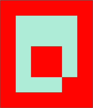

The two colours meet in a checkerboard pattern at the lower contact. The picture alone cannot say which diagonal should be connected.

Reconstruct without resolving the junction

Ordinary reconstruction closes the oriented ring at the diagonal contact. It then treats the identity-oriented interior and exterior as separate grains, so the map contains three grains rather than two.

grainsWithQuadruple = calcGrains(ebsd,'angle',10*degree);

fprintf('ordinary reconstruction: %d grains\n',length(grainsWithQuadruple))

grainColors = colorKey.orientation2color(grainsWithQuadruple.meanOrientation);
plot(grainsWithQuadruple,grainColors,'micronbar','off');
hold on
plot(grainsWithQuadruple.boundary,'lineWidth',2);
hold off

ordinary reconstruction: 3 grains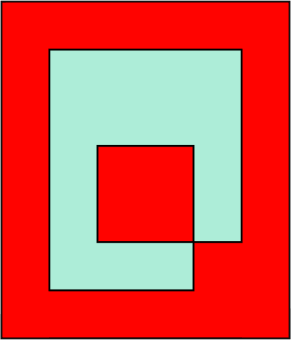

The interior patch has its own outline. At the diagonal contact, four thick boundary segments end at the same vertex.

Resolve the junction during reconstruction

The 'removeQuadruplePoints' option selects the other diagonal. It keeps the like-oriented interior and exterior connected; the ring pixels were already connected to each other elsewhere. The expected two grains remain.

grains = calcGrains(ebsd,'angle',10*degree,'removeQuadruplePoints');

fprintf('resolved reconstruction: %d grains\n',length(grains))
fprintf('total boundary length: %g before, %g after\n',...
  sum(grainsWithQuadruple.boundary.segLength),...
  sum(grains.boundary.segLength))
fprintf('strict triple points: %d\n',length(grains.triplePoints))

grainColors = colorKey.orientation2color(grains.meanOrientation);
plot(grains,grainColors,'micronbar','off');
hold on
plot(grains.boundary,'lineWidth',2);
hold off

resolved reconstruction: 2 grains
total boundary length: 52.0014 before, 52.0014 after
strict triple points: 0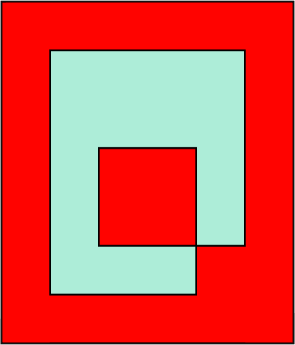

The interior outline has joined the exterior network, while the boundary segments and their total length are unchanged. Only their connectivity at the critical vertex differs.

The option replaces the four-segment vertex with two coincident three-segment junctions. In this two-grain example they are not strict triple points, because a triple point must separate three distinct real grains. See Triple Points for that distinction.

Separate the coincident junctions for display

The two replacement junctions initially have identical coordinates. smoothBoundary normally fixes every junction. Its 'moveTriplePoints' option releases every interior junction, despite the narrower name, and lets the two points move apart.

A taubinFilter suppresses the pixel staircase while limiting the systematic area loss of Laplacian smoothing.

grains = smoothBoundary(grains,taubinFilter,'moveTriplePoints');

grainColors = colorKey.orientation2color(grains.meanOrientation);
plot(grains,grainColors,'lineWidth',2,'micronbar','off');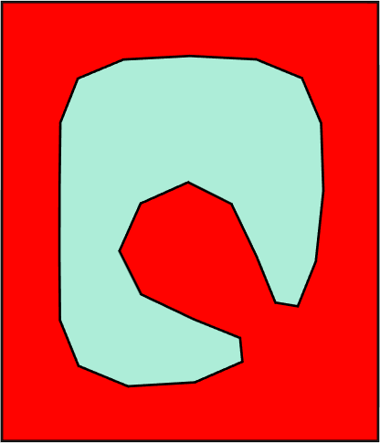

The coincident contact has opened into a narrow neck. Smoothing has moved the geometry for display; it did not perform the topological correction.

Curvature at the opened contact

Signed curvature makes the opened pinch visible as neighbouring bends in opposite directions.

gB = grains(1).boundary;

plot(gB,gB.curvature(10),'lineWidth',6,'micronbar','off');
mtexColorMap('blue2red');
setColorRange(0.5*[-1,1]);
mtexColorbar('title','signed curvature in 1/grid unit');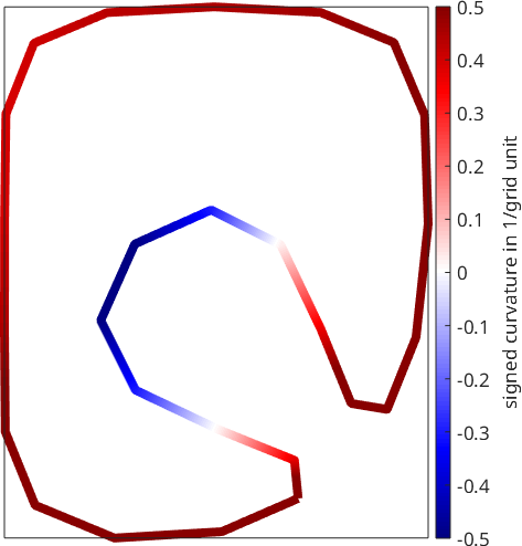

The blue and red extrema beside the pinch have opposite signs. The sign depends on the stored walk direction, so use Boundary Curvature before interpreting it as convex or concave relative to a particular grain.

References

Next

Continue with Boundary Intersections for geometric crossings between boundaries and other curves. For the two operations used here, see Grain Boundary Smoothing and Boundary Curvature.

References

- T. Y. Kong and A. Rosenfeld, Digital topology: Introduction and survey, Computer Vision, Graphics, and Image Processing 48 (1989), 357--393, develops the adjacency choices behind diagonal connectivity on a digital grid.
- C. Herring, Surface Tension as a Motivation for Sintering, in The Physics of Powder Metallurgy (1951), 143--179, gives the classical capillary balance at physical junctions.
- P. R. Rios and M. E. Glicksman, Grain boundary, triple junction and quadruple point mobility controlled normal grain growth, Philosophical Magazine 95 (2015), 2092--2127, distinguishes the roles of boundaries, triple junctions, and quadruple points in grain-growth models.