Three-Dimensional EBSD Analysis

Everything measured on a polished surface is a section through something three-dimensional, and a section is a biased witness. A section through a grain almost never passes through its widest part, so its apparent size is smaller than that grain's full extent. An elongated grain can look equiaxed when it is cut across rather than along its long direction, and the inclination of a grain boundary away from the section is lost altogether.

Three-dimensional data removes these compromises. It can come from serial sectioning, from diffraction techniques that probe a volume, or from a simulated microstructure. This page walks through the whole analysis on one such data set: import the volume, look at it, cut sections, reconstruct the grains, measure them, and smooth their boundaries. Every step has a page of its own in this chapter that treats it in depth.

plottingConvention.default('y↑→x');
how2plot = plottingConvention.default3D;

Import a volume

EBSD3.load reads a volume from a DREAM.3D file or from the Xnovo GrainMapper3D format and detects which of the two it is given. The sample data set is a simulated nine-phase volume in the Xnovo format, which mtexdata fetches by name.

ebsd = mtexdata('xnovo')

ebsd = EBSD3square (y↑→x)
 
 Phase  Orientations     Mineral          Color  Symmetry  Crystal reference frame
     0   27950 (22%)  notIndexed           none                                   
     1  11046 (8.8%)     Silicon        SkyBlue      m-3m                         
     2  11876 (9.5%)     Diamond  PaleVioletRed      m-3m                         
     3  10436 (8.3%)   Magnesium            Red     6/mmm        X||a, Y||b*, Z||c
     4  10231 (8.2%)      Rutile            Red     4/mmm                         
     5   9060 (7.2%)    Corundum    YellowGreen      -3m1        X||a, Y||b*, Z||c
     6  11521 (9.2%)      Quartz    DeepSkyBlue      -3m1        X||a, Y||b*, Z||c
     7  10961 (8.8%)    Pyroxene     SandyBrown       mmm                         
     8  10578 (8.5%)  Hornblende         Orchid     12/m1        X||a, Y||b, Z||c*
     9  11341 (9.1%)  Microcline           Gold        -1              X||a, Z||c*
 
 Properties: Completeness, grainId
 Scan unit : mm
 X × Y × Z : [-0.24 0.24] × [-0.24 0.24] × [-0.24 0.24]
 Grid size (square): 50 × 50 × 50

The summary reports a 50 x 50 x 50 array rather than a list: the measurements are held in an EBSD3 object whose entries are addressed as ebsd(i,j,k) along \(x\), \(y\) and \(z\). Each of the nine phases occupies about a twelfth of the voxels and the remaining fifth is not indexed. The voxel is 10 micron on a side and the volume spans half a millimetre in each direction.

[ebsd.dx, ebsd.dy, ebsd.dz]
ebsd.extent

ans =
    0.0100    0.0100    0.0100
ans =
   -0.2450    0.2450   -0.2450    0.2450   -0.2450    0.2450

Volume Data and Slices describes the object and its import in detail.

Display the volume

plot hands the volume to the MATLAB volume viewer, which cuts three slice planes through the data and lets you drag them, rotate, clip and crop with the mouse. It is a live window rather than a figure:

  plot(ebsd)

For a figure, cut the three central slices with slice and draw them into one axes. Each slice is an ordinary two-dimensional EBSD map, coloured by phase.

plot(slice(ebsd,plane3d(vector3d.Z,vector3d(0,0,0))),'micronbar','off')
hold on
plot(slice(ebsd,plane3d(vector3d.X,vector3d(0,0,0))),'micronbar','off')
plot(slice(ebsd,plane3d(vector3d.Y,vector3d(0,0,0))),'micronbar','off')
hold off
setCamera(how2plot)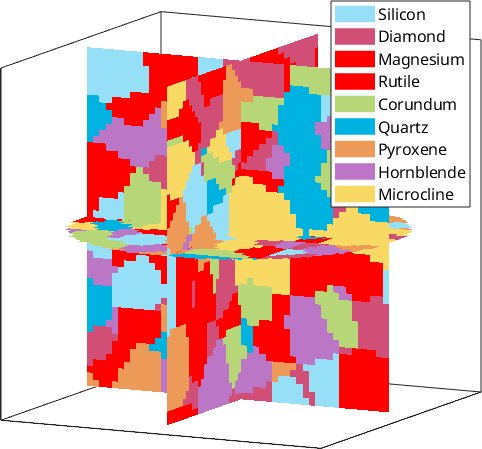

The specimen is a cylinder standing along \(z\): the horizontal section is a disc and the two vertical sections are rectangles that end at its rim. The nine phases are mixed through the volume without any layering.

Cut sections

A slice is taken through any plane, given by its normal and one point on it. The measurements of a section keep their position in the specimen, and the section is seen along the normal of the plane it was cut with, so an oblique cut displays like any other map.

newMtexFigure('layout',[1,2],'figSize','large');
plot(slice(ebsd,plane3d(vector3d.Z,vector3d(0,0,0.15))),'micronbar','off')
mtexTitle('normal || z, at z = 0.15 mm')
nextAxis
plot(slice(ebsd,plane3d(vector3d(1,1,1),vector3d(0,0,0))),'micronbar','off')
mtexTitle('normal || (1,1,1)')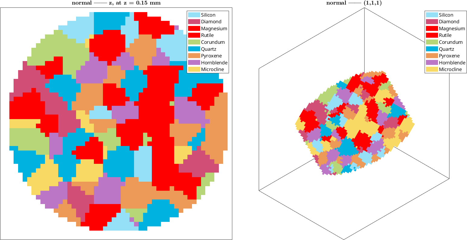

Everything written for planar data applies to a section unchanged. The quartz orientations of the oblique cut, for instance, are coloured with the usual inverse pole figure key.

ebsdCut = slice(ebsd,plane3d(vector3d(1,1,1),vector3d(0,0,0)));
plot(ebsdCut,ebsdCut.prop.Completeness,'facealpha',0.1)
mtexColorMap white2black
hold on
plot(ebsdCut('Quartz'),ebsdCut('Quartz').orientations,'micronbar','off')
hold off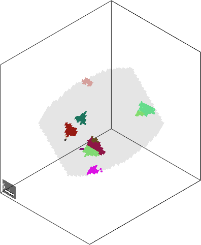

Volume Data and Slices shows slices at several depths and how a section relates to the volume it was cut from.

Reconstruct the grains

A grain is a connected region of voxels of one phase whose orientations differ by less than a threshold. calcGrains segments the volume with the same misorientation criteria as the planar case and returns a grain3d object. Where an EBSD3 holds one measurement per voxel, a grain3d holds each grain as a closed polyhedron: its faces carry the geometry, its phase and mean orientation describe the material inside. 'minPixel' dissolves grains of fewer than ten voxels into their neighbours; a grain that small is all corners and no surface.

[grains,ebsd] = calcGrains(ebsd,'angle',2*degree,'minPixel',10);
grains

grains = grain3d (y↑→x)
 
 Phase  Grains  Volume     Mineral  Symmetry  Crystal reference frame
     0       8   0.028  notIndexed                                   
     1      54   0.011     Silicon      m-3m                         
     2      58   0.012     Diamond      m-3m                         
     3      51    0.01   Magnesium     6/mmm        X||a, Y||b*, Z||c
     4      45    0.01      Rutile     4/mmm                         
     5      48  0.0091    Corundum      -3m1        X||a, Y||b*, Z||c
     6      52   0.012      Quartz      -3m1        X||a, Y||b*, Z||c
     7      56   0.011    Pyroxene       mmm                         
     8      49   0.011  Hornblende     12/m1        X||a, Y||b, Z||c*
     9      54   0.011  Microcline        -1              X||a, Z||c*
 
 boundary faces: 166738
 
 Properties: meanRotation, GOS

Voxels that are not indexed form regions of their own, which are listed as grains of the phase notIndexed. The indexed grains are selected the way a phase is selected on a map.

grains = grains('indexed');

Plotting the whole collection shows the outer surface of the volume, one colour per phase. Every grain behind it is present in the collection.

plot(grains,'micronbar','off','edgeAlpha',0.1)
setCamera(how2plot)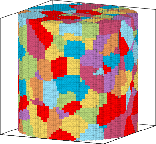

Individual grains are addressed by their id. The five largest grains of the volume, drawn together, show the surface a reconstruction from voxels produces: every face is a voxel face, so the surface is a staircase whose normals all point along the axes.

[~,order] = sort(grains.volume,'descend');
largest = grains(order(1:5))

plot(largest,'micronbar','off','edgeAlpha',0.2)
setCamera(how2plot)

largest = grain3d (y↑→x)
 
 Phase  Grains  Volume  Mineral  Symmetry  Crystal reference frame
     1       3  0.0017  Silicon      m-3m                         
     4       2  0.0011   Rutile     4/mmm                         
 
 boundary faces: 5496
 
  Id   Phase   Pixels      meanRotation       GOS
 473       1      585   (133°,29°,229°)         0
 148       4      562    (323°,73°,44°)         0
 470       1      553   (169°,27°,202°)         0
 463       4      550   (264°,90°,112°)         0
  48       1      550   (320°,20°,360°)   4.2e-08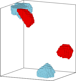

Grain Reconstruction explains the criteria, the 'minPixel' option and how to compare the result with the grain ids a file already carries. Three-Dimensional Grains imports a mesh from DREAM.3D instead of reconstructing one.

Measure the grains

A three-dimensional grain has a volume and a surface area, and neither needs a stereological correction. Volumes are in cubic millimetres here, the unit of the coordinates.

[largest.volume, largest.surface]

ans =
    0.0006    0.0564
    0.0006    0.0544
    0.0006    0.0578
    0.0006    0.0558
    0.0006    0.0514

The two combine into a dimensionless measure of compactness, the surface area divided by the volume to the power two thirds. A sphere gives the smallest possible value, \((36\pi)^{1/3} \approx 4.84\), a cube gives 6, and a grain with a rough or elongated surface gives more.

shapeQuotient = grains.surface ./ grains.volume.^(2/3);

histogram(shapeQuotient)
xlabel('surface / volume^{2/3}')
ylabel('number of grains')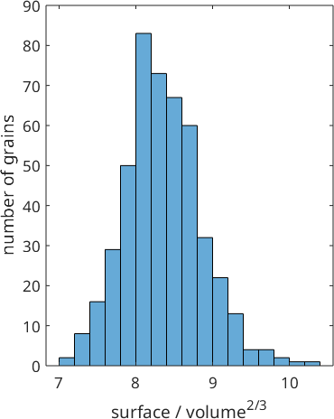

Every grain lies well above the cube's 6, although the grains are equiaxed and convex. The staircase inflates the surface: a voxel surface has the area of the axis-aligned faces it is made of, whatever shape it encloses. Sizes are unaffected, since the volume of a voxel grain is exact.

Properties covers diameters, principal axes, neighbours and the per-face properties of the boundary.

Smooth the boundaries

The staircase is removed in two steps. reduceBoundary merges the vertices of each voxel-sized cell of a coarser lattice, which already averages the steps and leaves a mesh a quarter the size. smoothBoundary then moves the vertices with one of the boundary filters of the planar case. Triple lines, quadruple points and the outer hull of the volume stay where they are, so the network keeps its topology.

grainsS = smoothBoundary(reduceBoundary(grains,2,'quadric'),taubinFilter(20));

plot(grainsS('id',largest.id),'micronbar','off','edgeAlpha',0.2)
setCamera(how2plot)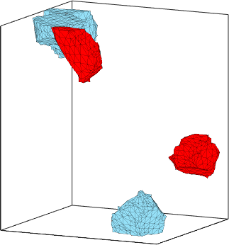

The same five grains are now bounded by smooth surfaces. The volume of the whole specimen is conserved exactly, since its hull is fixed. Between the grains and the unindexed regions between them a fraction of a percent moves, and the volume of a single grain changes by a few percent.

[sum(grains.volume), sum(grainsS.volume)]

ans =
    0.0970    0.0962

The compactness measure responds as it should: the surfaces lost their steps, and the histogram moves down towards the range between a sphere and a cube.

shapeQuotientS = grainsS.surface ./ grainsS.volume.^(2/3);

edges = 5:0.25:10.5;
histogram(shapeQuotient,edges,'DisplayName','voxel surface')
hold on
histogram(shapeQuotientS,edges,'DisplayName','smoothed')
hold off
legend('Location','northeast')
xlabel('surface / volume^{2/3}')
ylabel('number of grains')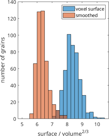

Smoothing compares the filters and the placement rules of the coarsening, with the volume they cost per grain. Boundary Network reads the faces, triple lines and quadruple points of the smoothed mesh, and Boundary Normal Distribution contrasts boundary normals measured from the faces with stereological estimates from traces.

Where to read on

Neper Interface generates a synthetic polycrystal or imports an existing .tess file, which gives a microstructure of known construction to test an analysis against. Operations traces planar sections back to their parent grains, triangulates polygonal faces and rotates a collection.

The two-dimensional foundations are developed in EBSD, Grains and Grain Boundaries.

References

Next

Continue with Volume Data and Slices, the first page of the chapter, and follow the sidebar from there.

References

- F. Bachmann, R. Hielscher, and H. Schaeben, Grain Detection from 2d and 3d EBSD Data - Specification of the MTEX Algorithm, Ultramicroscopy 111 (2011), 1720--1733, develops the spatial cells and connectivity used to define grains from two- and three-dimensional data.
- S. Maddali, S. Ta'asan, R. M. Suter, Topology-faithful nonparametric estimation and tracking of bulk interface networks, Computational Materials Science 125 (2016), 328--340, is the stratified smoothing scheme that keeps triple lines and quadruple points in place.
- M. A. Groeber and M. A. Jackson, DREAM.3D: A Digital Representation Environment for the Analysis of Microstructure in 3D, Integrating Materials and Manufacturing Innovation 3 (2014), 56--72, describes the data environment and surface-mesh representation of the other importer.