Grains

From an orientation map to grain objects

An orientation map tells you what the crystal lattice is doing at every measured point. It does not tell you where one crystal ends and the next one begins. Grain reconstruction makes that interpretation by grouping connected measurements according to phase and orientation.

This changes the questions the map can answer. A million measurements can become a few thousand grains, each with a size, shape, mean orientation, and list of neighbours. Questions about grain size, elongation, and contact only become answerable after the boundaries have been defined.

This chapter assumes that an EBSD map is familiar. Read Misorientation Theory first if the angle between two crystal orientations is new to you.

% draw the specimen with y up and x to the right
plottingConvention.default('y↑→x');
mtexdata forsterite silent

% restrict the map to a subregion of interest
ebsd = ebsd(inpolygon(ebsd,[5 2 10 5]*10^3));

% reconstruct grains and store each grain id with its measurements
[grains,ebsd] = calcGrains(ebsd('indexed'),'angle',10*degree);

% inspect the resulting grain list
grains

grains = grain2d (y↑→x)
 
 Phase  Grains  Pixels     Mineral  Symmetry         Color
     1     107   14093  Forsterite       mmm  LightSkyBlue
     2      32    1397   Enstatite       mmm  DarkSeaGreen
     3      71     759    Diopside     12/m1     Goldenrod
 
 boundary segments: 3921 (188891 µm)
 inner boundary segments: 1 (19 µm)
 triple points: 244
 
 Properties: meanRotation, GOS

The displayed grain2d summary is the first result of reconstruction. One object holds the complete grain list, and its methods act across that list. Its three phase rows contain 210 grain sections: 107 Forsterite, 32 Enstatite, and 71 Diopside. The second output above stores a persistent grainId with every EBSD measurement. A grain and its measurements can therefore be selected from either side of the relationship.

Here is that relationship in one picture. The coloured points are the measured Forsterite orientations. The black lines are the boundaries of every indexed grain, including grains of the other indexed phases.

plot(ebsd('Forsterite'),ebsd('Forsterite').orientations,...
  'ipfDirection',zvector,'micronbar','off')
hold on
plot(grains.boundary,'lineWidth',1.5)
hold off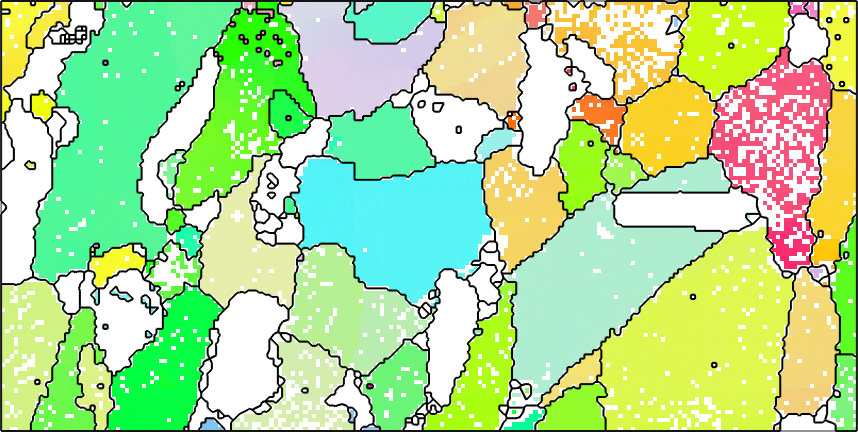

Follow one black line through the map. It runs along the interfaces between neighbouring spatial cells assigned to different grains. This is why the line looks stepped when you zoom in. Smoothing is a later measurement decision, not part of reconstruction or a recovery of the unmeasured sub-pixel interface.

White inside the cropped map is not automatically notIndexed. The plot only colours Forsterite, whereas the black network includes every indexed phase. A Forsterite measurement with no finite orientation also plots white.

The words used in this chapter

Grain - a phase-homogeneous, spatially connected region of EBSD pixels produced by segmentation. A phase change between neighbouring pixels is always a grain boundary, so orientation-based segmentation never joins two phases into one grain.

The angle criterion is local. It decides whether neighbouring pixels of one phase are connected. A chain of accepted neighbours can accumulate orientation change, so two distant pixels in one grain may differ by more than the segmentation angle.

A grain2d object describes the section of a grain in the map plane. It is not the complete three-dimensional grain. Inferring three-dimensional size or shape from such sections requires a stereological model.

notIndexed - the phase given to a recorded measurement whose diffraction pattern could not be indexed. A connected notIndexed area can form its own grain. A patch that is too small or thin to stand alone may instead be absorbed into a neighbouring grain according to the 'alpha' setting. It is a failed indexing result, not an absent scan position.

Grain boundary - a segment between neighbouring EBSD pixels assigned to different grains. The segments are stored as a grainBoundary object with its own properties and its own chapter. A phase boundary is not another kind of object. It is a grain boundary whose two neighbouring grains have different phases.

Enclosure - the relationship in which one grain lies entirely inside another. Seen from outside, the containing grain has a hole. Seen from inside, the contained grain is an inclusion. These are the same fact from opposite sides, and the hole is never empty: even a notIndexed patch is itself a grain.

Recommended reading order

Begin with Reconstruction. It explains the segmentation angle, notIndexed measurements, and the minimum grain size. These choices shape every quantity computed afterwards.

Continue with Plot and Select. The second page distinguishes persistent grain IDs from positions in a shortened or reordered grain list.

The shape route begins with Shape Parameters for direct measurements such as area, perimeter, and diameter. Read Smoothing before interpreting outline length, direction, or curvature. The next pages replace each outline by a simpler description: an ellipse, a convex hull, or directional projections. Each preserves different information, so choose according to the expected shape.

Orientation Parameters describes the mean orientation and the orientation spread inside each grain. Dispersion Axes develops a validation workflow for grains whose orientations appear to follow one dominant rotation. Both build on misorientation rather than boundary shape.

Neighbours changes from a list of grains to their contact network. Merge then removes selected internal boundaries, for example between a host and a twin domain. The merge page assumes Boundary Misorientations, so visit that page in the next chapter before returning.

For segmentation that a single hard angle cannot describe, continue with Advanced Reconstruction and then Markovian Clustering. The latter requires the weighted criteria introduced by the former.

Finish with Export. It explains which parts of a grain object survive each exchange format. Neper Interface then connects MTEX grain sections to synthetic polycrystal generation.

Why the segmentation angle is a decision

There is no canonical grain reconstruction for every material. A grain in a textbook is a volume of material with a continuous lattice. An EBSD map samples orientations on a plane, so converting those samples into regions requires a rule chosen for the analysis.

Angles of 10 or 15 degrees are long-standing conventions for separating low- and high-angle boundaries. The Read-Shockley model explains why the energy of a simple low-angle boundary rises with misorientation, but the transition and high-angle energy depend on material and boundary character. The chosen angle is therefore not an independently measured specimen value.

Deformed material makes the choice especially visible. A bent lattice can accumulate orientation change gradually, so one angle may keep it whole while another splits it into several grains. The literature supports more than one useful grain definition, which is why Advanced Reconstruction and Markovian Clustering offer different answers rather than a universal fix.

What a two-dimensional boundary leaves unknown

A physical interface is a structure a few atoms thick. Its macroscopic crystallographic character takes five parameters: three for the misorientation between the crystals and two for the interface-plane normal.

A polished two-dimensional map supplies the misorientation and the trace where the interface cuts the surface. It does not supply the inclination of each interface plane. Recovering that missing parameter requires 3D data, or a stereological estimate from many boundary traces rather than a claim about one segment.

References

Next

Grains come from an orientation map, so EBSD is the preceding chapter. Their segments, chains, and junctions are the subject of the next chapter, Grain Boundaries. To analyse a distribution of grain mean orientations, return to ODF.

References

- F. Bachmann, R. Hielscher, and H. Schaeben, Grain Detection from 2d and 3d EBSD Data - Specification of the MTEX Algorithm, Ultramicroscopy 111 (2011), 1720--1733. This paper derives the spatial cells, connectivity, grains, and boundaries used by
calcGrains.
- F. J. Humphreys, Grain and Subgrain Characterisation by Electron Backscatter Diffraction, Journal of Materials Science 36 (2001), 3833--3854. This review compares useful grain definitions and shows why deformed microstructures separate them.
- W. T. Read and W. Shockley, Dislocation Models of Crystal Grain Boundaries, Physical Review 78 (1950), 275. This paper develops the classic low-angle boundary-energy model.
- A. P. Sutton and R. W. Balluffi, Interfaces in Crystalline Materials, Clarendon Press, 1995. This textbook develops the structure, thermodynamics, kinetics, and properties of interfaces.
- C.-S. Kim, A. D. Rollett, and G. S. Rohrer, Grain Boundary Planes: New Dimensions in the Grain Boundary Character Distribution, Scripta Materialia 54 (2006), 1005--1009. It explains the five-parameter description and what a planar EBSD map can observe.
- ISO 13067:2020, Microbeam Analysis - Electron Backscatter Diffraction - Measurement of Average Grain Size. The standard distinguishes measurements on a two-dimensional section from inferred three-dimensional grain size and cautions against uncritical interpretation of highly deformed material.