Grain Reconstruction by Markovian Clustering edit page

Once the grain boundary criterion has judged every pair of neighbouring pixels, the grains still have to be read off. By default they are the connected components of the pairs that were not separated - two pixels end up in the same grain whenever any chain of unseparated pairs leads from one to the other, however long and however thin. This makes the reconstruction a local decision taken by the weakest link: a single chain of pixels that just missed the threshold merges two grains, and no amount of evidence along the rest of the boundary can outvote it.

The Markovian clustering algorithm (MCL) replaces this all or nothing rule by a flow computation on the same graph, in which every pair takes part with the weight the criterion gave it. It is selected by the option 'mcl', whose value is the pair [p maxIter] of the inflation power and the number of iterations.

Flow simulation on the pixel graph

Think of the map as a graph whose nodes are the pixels and whose edges join neighbouring pixels, each edge carrying the connectivity w between 0 and 1 that the criterion returned for that pair. Normalising the weights of the edges leaving a pixel turns this graph into a Markov chain: a random walker sitting on a pixel hops to one of its neighbours with a probability proportional to the connectivity between them, so it crosses a well connected pair often and a poorly connected one rarely.

The observation MCL is built on is that such a walker gets trapped. A grain is an area the walker can move around in freely, while the boundary around it is a bottleneck of low probability edges - so a walk that starts inside a grain is, after a few steps, still overwhelmingly likely to be inside the same grain. Grains are thus the regions the flow does not leave, and the algorithm finds them by making that statistical preference absolute. Writing A for the column normalised transition matrix it alternates two operations:

  • expansion, A = A^2, which lets the walk take twice as many steps as before and so spreads the flow further into the region around each pixel
  • inflation, A = A.^p followed by a renormalisation of every column, which raises the probabilities to the power of the inflation power p and thereby strengthens the steps that were already likely at the expense of the unlikely ones

Expansion lets a pixel see further and further into its neighbourhood, inflation removes what the walk found unattractive. Repeated, the two drain the flow out of the bottlenecks entirely: the transition matrix falls apart into blocks with no probability left in between, and those blocks are the clusters. The algorithm is due to Stijn van Dongen, who introduced it in his thesis Graph Clustering by Flow Simulation (University of Utrecht, 2000) and later published it as Graph clustering via a discrete uncoupling process (SIAM J. Matrix Anal. Appl. 30(1):121-141, 2008).

Note that nothing in this asks what the weights mean. MCL takes the weights of whatever criterion produced them, including gbcCustom and criteria of your own, and clusters them.

What MTEX does differently

MCL was designed for abstract similarity graphs, in which any node may be linked to any other. Here the graph is a map: a pixel is joined to its immediate neighbours and to nothing else, the matrix is extremely sparse and, more importantly, the clusters that are looked for are connected regions of the specimen surface. The implementation in MTEX makes use of this in three places.

The flow is confined to the pixel graph. Entries that fall below 1e-4 are pruned after every inflation, which keeps the matrix sparse even though expansion by squaring fills it in; and a self loop is put on every pixel, so that a walker may also stay where it is, which keeps the flow from oscillating back and forth between neighbours instead of settling.

The iteration count is a length scale, not a convergence budget. Each expansion squares the matrix and so doubles the length of the walk, which means that after a handful of iterations a pixel already sees a neighbourhood tens of pixels wide - the scale on which the clusters are eventually decided. Van Dongen's algorithm is run until the matrix stops changing; MTEX stops it after maxIter cycles, four by default, and the number matters. Left to converge on the map below it does what it is supposed to do and concentrates the flow on individual attractors, returning 1638 clusters where four iterations return 136.

The clusters are read off geometrically. Instead of interpreting the converged matrix, MTEX takes the connected components of the flow that survived, and draws a grain boundary between every pair of neighbouring pixels whose flow died. The result is a grain2d object like any other, with a complete boundary network, and all of grain reconstruction applies to it unchanged.

Why the criterion has to be soft

MCL works on the weights of the graph, so it needs a criterion that produces more than yes and no. With the default threshold criterion every weight is 0 or 1, the walk cannot distinguish a weak connection from a strong one, and MCL returns exactly the connected components it would have returned anyway - only much slower.

We demonstrate this on the deformed austenite of the EMSphinx data set, the same one the basic page uses.

plottingConvention.default("y↓→x");
mtexdata EMSphinx silent

ebsd = ebsd('Iron fcc');
ebsd = ebsd(inpolygon(ebsd,[40 30 80 60]));

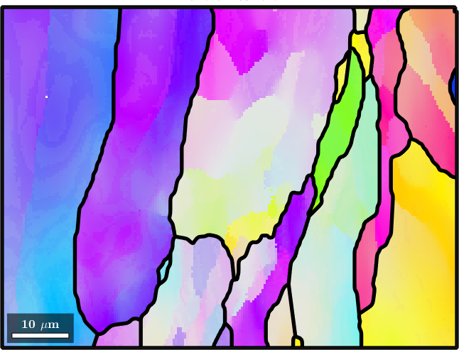
grains = calcGrains(ebsd,'angle',10*degree,'minPixel',10)
grains = smoothBoundary(grains,5);

plot(ebsd,ebsd.orientations)
hold on
plot(grains.boundary,'LineWidth',4)
hold off
grains = grain2d (y↓→x)
 
 Phase  Grains  Pixels   Mineral  Symmetry         Color
     1      19   29989  Iron fcc      m-3m  DarkSeaGreen
 
 boundary segments: 2137 (853 µm)
 inner boundary segments: 126 (50 µm)
 triple points: 20
 
 Id   Phase   Pixels       meanRotation      GOS
  1       1     6218   (341°,115°,219°)    0.059
  2       1      196   (132°,147°,125°)    0.019
  3       1       37    (108°,54°,291°)   0.0081
  4       1     5199   (329°,118°,120°)    0.061
  5       1       58    (93°,141°,142°)    0.012
  6       1     1489    (279°,35°,331°)    0.087
  7       1      250     (86°,153°,21°)    0.047
  8       1       18     (96°,25°,183°)   0.0089
  9       1     1261    (136°,35°,230°)     0.09
 10       1       75     (268°,93°,64°)   0.0067
 11       1     6046    (68°,149°,118°)     0.11
 12       1      623   (112°,142°,273°)    0.019
 13       1       71   (126°,151°,198°)    0.016
 14       1      120    (177°,65°,272°)     0.02
 15       1     2530    (195°,57°,283°)    0.071
 16       1     1334    (87°,159°,223°)     0.11
 17       1       34   (275°,126°,229°)   0.0083
 18       1     1574     (212°,17°,25°)    0.057
 19       1     2856   (124°,156°,355°)    0.052

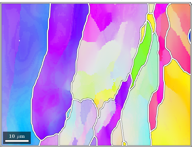
Adding 'mcl' to this call changes nothing - the same 19 grains with the same 2137 boundary segments, at any inflation power one cares to try, so the white lines cover the black ones exactly.

grains = calcGrains(ebsd,'mcl',[1.6 4],'angle',10*degree,'minPixel',10)
grains = smoothBoundary(grains,5);

hold on
plot(grains.boundary,'LineWidth',3,'LineColor','White')
hold off
grains = grain2d (y↓→x)
 
 Phase  Grains  Pixels   Mineral  Symmetry         Color
     1      19   29989  Iron fcc      m-3m  DarkSeaGreen
 
 boundary segments: 2137 (853 µm)
 inner boundary segments: 110 (44 µm)
 triple points: 20
 
 Id   Phase   Pixels       meanRotation      GOS
  1       1     6218   (341°,115°,219°)    0.059
  2       1      196   (132°,147°,125°)    0.019
  3       1       37    (108°,54°,291°)   0.0081
  4       1     5199   (329°,118°,120°)    0.061
  5       1       58    (93°,141°,142°)    0.012
  6       1     1489    (279°,35°,331°)    0.087
  7       1      250     (86°,153°,21°)    0.047
  8       1       18     (96°,25°,183°)   0.0089
  9       1     1261    (136°,35°,230°)     0.09
 10       1       75     (268°,93°,64°)   0.0067
 11       1     6046    (68°,149°,118°)     0.11
 12       1      623   (112°,142°,273°)    0.019
 13       1       71   (126°,151°,198°)    0.016
 14       1      120    (177°,65°,272°)     0.02
 15       1     2530    (195°,57°,283°)    0.071
 16       1     1334    (87°,159°,223°)     0.11
 17       1       34   (275°,126°,229°)   0.0083
 18       1     1574     (212°,17°,25°)    0.057
 19       1     2856   (124°,156°,355°)    0.052

What the weights have to encode is the ambiguity of the data, and in a deformed material there is plenty of it. The misorientation between neighbouring pixels of this map has no gap anywhere: it runs continuously from the noise floor of the indexing, through the bent lattice inside the grains, into the subgrain boundaries and on to the high angle boundaries.

ori = ebsd.gridify.orientations;
omega = [reshape(angle(ori(1:end-1,:),ori(2:end,:)),[],1); ...
  reshape(angle(ori(:,1:end-1),ori(:,2:end)),[],1)];
omega(isnan(omega)) = [];

close all
histogram(omega./degree,0:0.05:3)
xlabel('misorientation angle to the neighbouring pixel in degree')

The narrow peak at 0.15 degree is the noise floor of the indexing, the broad shoulder around 0.8 degree the subgrain boundaries we are after - and between the two there is no empty range to put a threshold into. Half of the pairs stay below 0.23 degree and are plainly inside a grain, 2.6 percent are above 10 degree and plainly are not, and the quarter in between is what the reconstruction has to decide.

quantile(omega./degree,[0.5 0.75 0.9 0.95])
ans =
    0.2298
    0.4926
    0.9399
    1.9975

The soft threshold gbcSoft hands that decision on instead of taking it. Its connectivity is an error function rather than a step, so a pair in the ambiguous band gets a weight strictly between 0 and 1 - the more suspicious the misorientation, the thinner the flow that is allowed through it. It is passed by the option 'soft' as a pair [angle width], and both entries matter. The centre angle is where the weight passes through one half and belongs where the histogram is ambiguous - here half a degree, above the noise peak and below the subgrain shoulder. The width decides how much of that band is graded rather than decided, and should be of the same order as the centre: a width much smaller makes the error function steep again, which is a hard threshold in disguise and of no use to MCL.

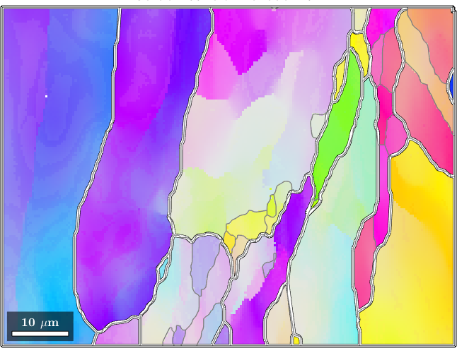
On its own the soft criterion is still evaluated by connected components, so all it can do is move the threshold. It finds a few of the low angle boundaries the 10 degree threshold missed - 43 grains instead of 19 - but not the substructure inside the elongated grains. What it does record are the 12621 inner boundary segments: pairs in the transition band that were suspicious enough to draw a boundary, but did not manage to separate anything.

grains = calcGrains(ebsd,'soft',[0.5 0.5]*degree,'minPixel',10)
grains = smoothBoundary(grains,5);

plot(ebsd,ebsd.orientations)
hold on
plot(grains.boundary,'LineWidth',1.5)
hold off
grains = grain2d (y↓→x)
 
 Phase  Grains  Pixels   Mineral  Symmetry         Color
     1      43   29961  Iron fcc      m-3m  DarkSeaGreen
 
 boundary segments: 2767 (1104 µm)
 inner boundary segments: 12621 (5048 µm)
 triple points: 63
 
 Properties: meanRotation, GOS

The reconstruction

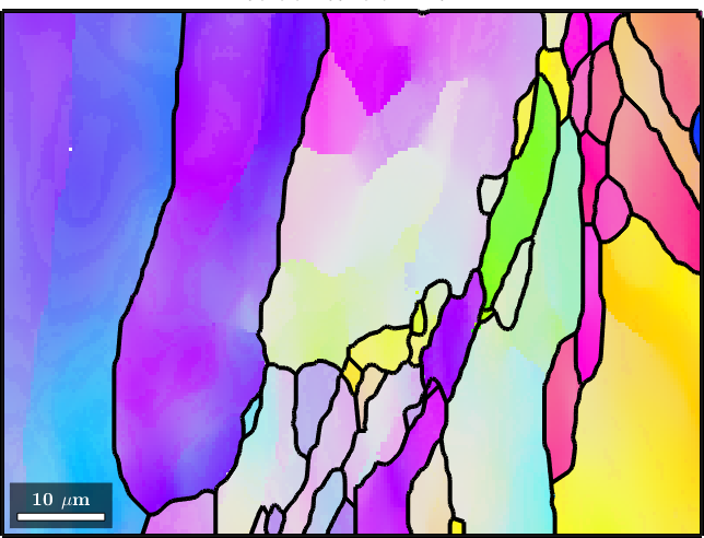
Handing the same weights to MCL changes the answer. The flow computation is not impressed by a chain of mildly suspicious pairs running through the interior of a grain, but it is by a coherent line of them that surrounds a region.

grains = calcGrains(ebsd,'mcl',[1.6 4],'soft',[0.5 0.5]*degree,'minPixel',10)
grains = smoothBoundary(grains,5);

plot(ebsd,ebsd.orientations)
hold on
plot(grains.boundary,'linewidth',1.5)
hold off
grains = grain2d (y↓→x)
 
 Phase  Grains  Pixels   Mineral  Symmetry         Color
     1     113   29177  Iron fcc      m-3m  DarkSeaGreen
 
 boundary segments: 4523 (1780 µm)
 inner boundary segments: 5140 (2041 µm)
 triple points: 155
 
 Properties: meanRotation, GOS

The low angle boundaries the 10 degree threshold missed are found, together with much of the substructure the deformation produced inside the elongated grains, and the smoothly bent lattice is left in one piece - which is what a threshold of half a degree did to it above.

Checking the result against the KAM map

Whether the flow was pinched off in the right places is hard to judge on an orientation map, where a subgrain boundary is a slight change of colour. The kernel average misorientation shows the same information as lines: every boundary, at whatever angle, is a ridge in it. Plotting the reconstruction on top of the KAM map is therefore the quickest way to see which boundaries the clustering picked up and which it walked past.

ebsdG = ebsd.gridify;
kam = KAM(ebsdG,'threshold',5*degree)./degree;

plot(ebsdG,kam)
mtexColorMap white2black
setColorRange([0 1.5])
mtexColorbar('title','KAM in degree')
hold on
plot(grains.boundary,'linewidth',1.5,'lineColor','red')
hold off

Most of the ridges carry a red line, but one does not: the long, sharp, almost vertical boundary in the left third of the map runs from the top edge to the bottom without being reconstructed. It is not a faint feature - the misorientation across it is 2 to 5 degrees, several times what the soft threshold is centred on.

The reason is the one the introduction warned about, and it is worth looking at closely, because it is what separates a clustering from a connected component analysis. The subgrain this boundary encloses turns out to be bounded by 258 pixel pairs. Of those, 240 carry a weight below 0.1 and are the boundary proper, 17 sit at about 0.7 degree and keep weights between 0.1 and 0.2 - and one single pair, somewhere along the line, is 0.2 degree apart, an entirely ordinary connection of weight 0.95. Connected components, whatever criterion they are given, cannot separate a region across one sound connection, and this is why the soft criterion above did not draw this boundary either. MCL can, but only if the inflation is sharp enough that the flow through that pair does not survive four rounds of squaring and renormalising - and at p = 1.6 it survives.

Raising the inflation power settles it.

grains = calcGrains(ebsd,'mcl',[1.8 4],'soft',[0.5 0.5]*degree,'minPixel',10)
grains = smoothBoundary(grains,5);

plot(ebsdG,kam)
mtexColorMap white2black
setColorRange([0 1.5])
mtexColorbar('title','KAM in degree')
hold on
plot(grains.boundary,'linewidth',1.5,'lineColor','red')
hold off
grains = grain2d (y↓→x)
 
 Phase  Grains  Pixels   Mineral  Symmetry         Color
     1     136   28787  Iron fcc      m-3m  DarkSeaGreen
 
 boundary segments: 5495 (2157 µm)
 inner boundary segments: 4997 (1986 µm)
 triple points: 177
 
 Properties: meanRotation, GOS

The boundary is now followed along its whole length. Measured over probe points on either side of it, p = 1.6 cuts it in 29 percent of the rows of the map and p = 1.8 in 89 percent - for comparison, gbcFMC reaches 79 percent and the soft criterion on its own, being a connected component analysis, reaches zero. On the orientation map this is the final reconstruction.

plot(ebsd,ebsd.orientations)
hold on
plot(grains.boundary,'linewidth',1.5)
hold off

The inflation power

Of the two parameters the inflation power is the one to turn. It sets how sharply the walk is forced onto its likely steps, so a larger value lets less flow survive and breaks the map into more and smaller clusters.

for p = [1.2 1.4 1.6 1.8 2.0]

  grains = calcGrains(ebsd,'mcl',[p 4],'soft',[0.5 0.5]*degree,'minPixel',10);
  fprintf('inflation %.1f: %d grains\n',p,length(grains));

end
inflation 1.2: 60 grains
inflation 1.4: 82 grains
inflation 1.6: 113 grains
inflation 1.8: 136 grains
inflation 2.0: 176 grains

The useful range is narrow and the ends of it are unmistakable. Below p = 1.2 too much flow survives, the segmentation falls back onto a connected component analysis of the weighted graph and returns the barely 50 grains the soft criterion produced on its own. Beyond p = 2 the grains start to shatter, at p = 3 into single pixels. What is worth trying lies between 1.2 and 2.

Note that the grain count alone is a poor guide within that range - it grows smoothly, while the question whether a particular boundary is pinched off or leaks is decided somewhere along the way. The KAM overlay of the previous section is the better instrument: raise p until the boundaries you can see are followed, and stop before boundaries appear where the map shows none.

The number of iterations

The iteration count acts in the same direction, since letting the walk spread further and inflating what it found again gives the flow another chance to die. It is the more expensive of the two, because every expansion squares the transition matrix and fills it in.

for maxIter = [2 4 6 8]

  tic;
  grains = calcGrains(ebsd,'mcl',[1.4 maxIter],'soft',[0.5 0.5]*degree,'minPixel',10);
  fprintf('%d iterations: %4d grains, %.1f seconds\n',...
    maxIter,length(grains),toc);

end
2 iterations:   53 grains, 0.2 seconds
4 iterations:   82 grains, 0.7 seconds
6 iterations:  127 grains, 1.7 seconds
8 iterations:  159 grains, 3.0 seconds

Since the two parameters do much the same thing, and only one of them costs anything, the advice is to leave maxIter at its default of 4 and to look for the segmentation by the inflation power. Note that this is not a truncated approximation of some correct answer that more iterations would reach - as the section above explains, running MCL to convergence here shatters the map, and the four iterations are the statement that grains are decided on the scale of a few tens of pixels.

When to use it

MCL is a global criterion: it does not ask about a pair of pixels in isolation but about how the whole map hangs together. On deformed material, where no single threshold angle works, that is exactly what is needed - but it is not the only way to get it. gbcFMC, described on the basic page, reaches a comparable segmentation of this same map - 107 grains at cmaha = 1.5 against the 136 here - at a comparable cost, both of them a second or two on this region and around twenty on the full map. Since it needs no threshold angle at all and leaves only one number to choose, it is the shorter road if all that is wanted is a reconstruction of a deformed microstructure.

What MCL offers instead is that the clustering and the criterion are independent of each other. It clusters the weights of any criterion, including one written for a property that has nothing to do with orientation, and it is the only way in MTEX to turn such a criterion into something better than a connected component analysis.