Orientation Distribution Functions

Crystallographic texture is the distribution of crystal orientations in a specimen. A measured orientation list says what was observed, but an orientation distribution function (ODF) describes the population as a continuous density over orientation space.

This chapter assumes that an orientation maps the crystal frame into the specimen frame. Review Orientation Theory and Orientation Symmetry if that map or its symmetry-equivalent representatives are not yet familiar.

Density is the central idea. In the continuous model, the volume fraction at one exact orientation is zero, just as the fraction of people who are exactly 180 centimetres tall is zero. A material fraction comes from integrating the ODF over a region of orientations.

MTEX reports density in multiples of a random distribution (mrd). A uniform texture is 1 mrd everywhere. A value of 20 mrd means that the density near that orientation is twenty times the random reference, not that 20 percent of the material has that exact orientation.

plottingConvention.default('y↑→x');

From Measured Orientations to a Density

The same EBSD data are shown below as discrete points and as a density. calcDensity places a kernel around each measured orientation. plotPDF then projects the estimated ODF into a pole density figure for the crystal direction h.

mtexdata forsterite silent
ori = ebsd('Forsterite').orientations;

odf = calcDensity(ori,'halfwidth',10*degree);
h = Miller(1,0,0,ori.CS);

plotPDF(odf,h,'contourf','figSize','small')
hold on
plotPDF(ori(1:200:end),h,'MarkerSize',3, ...
  'MarkerFaceColor','k','MarkerEdgeColor','k')
hold off
mtexColorbar('title','mrd')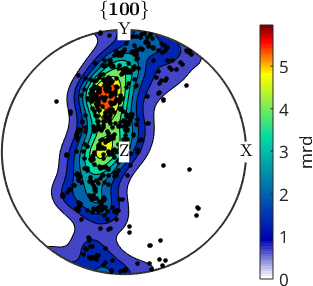

Each black dot is the specimen direction of h for one orientation in a regular subsample. The dots gather along a single high-density band. The band leaves the disc at one point of the rim and returns at the opposite point, because a pole figure identifies opposite directions and its rim is glued to itself. Isolated dots remain outside the filled contours, because the colours show a smoothed estimate rather than an outline around every observation.

The step from dots to colours requires a smoothing scale. The halfwidth states how far each measurement is spread through orientation space. Too small a halfwidth gives a bumpy record of the particular sample. Too large a halfwidth flattens real peaks. No value is correct independently of the data; Density Estimation develops this choice.

A second choice is what should count once. Pixel orientations weight the scanned area when the pixels have equal area. Grain mean orientations weight grains equally unless grain areas are supplied with the 'weights' option. Both choices are useful, but they answer different physical questions.

A Function on Rotations, Not on a Sphere

An ODF lives on the set of rotations. This space is three-dimensional and curved, so it has no faithful picture on a flat page. Every ODF figure is therefore a view with a specific loss of information.

A pole figure integrates the ODF along an orientation fibre. An inverse pole figure exchanges the chosen crystal and specimen directions. A section evaluates a two-dimensional slice and hides density away from that slice. These plots can resemble one another while answering different questions.

Crystal symmetry identifies equivalent numerical rotations exactly as it does for a single orientation. Specimen symmetry may identify further copies, but it should only be imposed when the specimen supports that assumption. Equivalent copies are not additional material.

Recommended Reading Order

Begin with Theory for the normalization and the density-versus-volume distinction. If the ODF comes from measured orientations, read Density Estimation next. Calculations then builds uniform, unimodal, and fibre ODFs with known answers.

Plot compares the available views. Continue in the order used by the chapter contents: Pole Figures, Inverse Pole Figures, Euler Angle Sections, and Sigma Sections. Conventional \(\varphi_2\) sections are compact for many cubic rolling textures. Sigma sections are often easier to interpret for trigonal, tetragonal, and hexagonal crystals because each panel reads like a pole figure of one chosen crystal axis, with the panel angle recording the remaining rotation about that axis.

After the section pages, Components locates and partitions modal populations. Properties extracts texture index, entropy, modes, and volume fractions. These are the scalar quantities most papers report when they compare textures.

The remaining pages are branches rather than one linear course. Shapes compares kernels; read it before Radial ODFs, whose components are sums of those kernels. Fibre ODFs spreads density along a curve, while Bingham ODFs fits a parametric statistical model. Series Expansion explains harmonic coefficients, bandwidth, and approximation. These representations share the SO3Fun interface, but differ in storage cost and in how efficiently they represent sharp features.

Import and Export handle files. Random Sampling turns a continuous ODF back into a finite orientation list, the reverse direction from density estimation. Sample Symmetry aligns an assumed specimen symmetry and explains why that alignment is not proof that the symmetry exists.

Further Reading

Next

ODFs are estimated from maps in EBSD and reconstructed from diffraction data in Pole Figures. The general machinery behind them is Orientation Functions. Using an ODF to predict a material property is covered in Tensors and Elasticity.