Orientation Functions

What is a function on rotations?

A function on rotations assigns a value to every rotation in \(\mathrm{SO}(3)\). Its value may describe a density, a physical response, or another quantity that changes as a crystal turns.

An orientation density function (ODF) is the most familiar example. A misorientation distribution is another. So are the Schmid factor of a slip system as the crystal turns and the stiffness of a grain along a fixed specimen direction.

This chapter treats the machinery shared by all these functions. The ODF chapter instead treats texture: what a density means, how to estimate it, and how to read its plots. Keeping the physical interpretation separate from the function representation makes both easier to follow.

Here the questions are how a function is stored, what evaluation costs, how samples can approximate it, and what rotation, differentiation, and convolution do to it.

A first picture

A function on rotations has a three-dimensional curved domain. A flat figure must therefore show cuts through it. The example below uses sigma sections, which hold the difference \(\sigma=\varphi_1-\varphi_2\) of the first and third Bunge angle fixed in each panel.

plottingConvention.default('y↑→x');

cs = crystalSymmetry('432');
mode = orientation.byEuler(30*degree,50*degree,10*degree,cs);
odf = unimodalODF(mode,'halfwidth',15*degree);

plot(odf,'sigma','sections',6,'figSize','medium')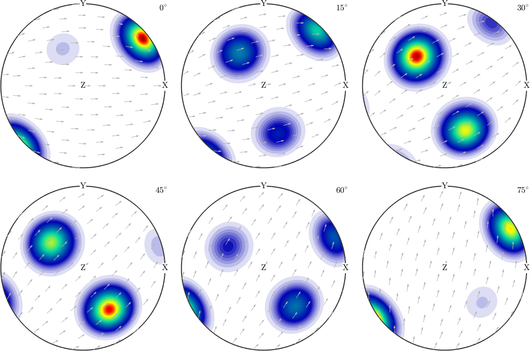

The six panels are slices through one function, not six different functions. A single peak appears in several panels because adjacent slices intersect the same three-dimensional feature. Every plot of a rotational function makes a comparable compromise.

Why rotations are harder than the sphere

A function on the sphere has a two-dimensional domain. A function on rotations has a three-dimensional domain, so its storage, evaluation, and visualization generally cost more.

Rotation space also closes up on itself in a way that has no two-dimensional analogue. No single flat picture can show it without cuts, and rotations that look far apart in Euler angles can be neighbours.

Symmetry folds the domain further. A function of crystal orientations is invariant under crystal symmetry acting on one side. If the specimen has symmetry, it is invariant under that symmetry acting on the other side. A texture therefore lives on a smaller, folded part of the rotation group, whose shape depends on both point groups.

Harmonic representations use the Wigner-D functions, defined on the closing page of this chapter. They are the rotational counterpart of spherical harmonics. Bandwidth has the same meaning in both settings, but the number of rotational coefficients grows with the cube of the bandwidth rather than the square.

Learn the common interface first

Begin with Concept, which explains the domain, symmetry, and available representations. Then use Definition to construct harmonic, radial basis, fibre, and Bingham functions. Operations covers evaluation, arithmetic, rotation, differentiation, and integration.

See the function

Plotting gives the overview. The two main families of slices are Sigma Sections and Euler Angle Sections. These pages are shared with the ODF chapter because plotting depends on the function, not on the physical meaning assigned to it.

Approximate a function from data

Approximation from data is the chapter's longest thread. Its pages share one aim but use different methods. Interpolation is the overview. Harmonic Interpolation fits harmonic coefficients, while RBF-Kernel Interpolation fits a sum of localized bumps.

Approximation and Quadrature develops the numerical integration behind these methods. It explains how finitely many samples can approximate an integral over rotations, which is neither obvious nor cheap.

Choose a representation

The representations have pages of their own: Harmonic Representation, Radial Basis Functions, Fibre Functions, and Bingham ODF.

Rotational Kernel Functions and Wigner-D Functions are their building blocks. Convolution joins functions for operations such as smoothing and the step from measurements to a density.

Symmetry, vector values, and files

Symmetry makes the folding of rotation space explicit.

Not every rotational function is scalar-valued. Vector Valued Functions covers arrays of values, and Rotational Vector Fields covers directions attached to the domain. A rotational vector field can express a texture's response to deformation by assigning each orientation the direction in which it is being turned.

Import and Export handle files.

Related foundations

For the physical meaning of a texture density, see ODF. The two-dimensional relatives are introduced in Spherical Functions. The underlying geometry is developed under Rotations and Orientations.

References

Next

Continue with Concept to distinguish a rotational function's domain, values, symmetries, and numerical representation before constructing one.

References

- H.-J. Bunge, Texture Analysis in Materials Science: Mathematical Methods, Butterworths, 1982, develops the orientation-space, symmetry, and harmonic framework summarized here.