Spherical Functions

A great deal of texture analysis attaches one value to every direction. A pole figure assigns an intensity to each specimen direction. Wave speed through a crystal, the density of measured axes, and the Schmid factor of a slip system under a rotating load are further examples. Each is a function on the sphere.

Treating these as one kind of object gives them a common set of operations. You can add two functions, take a maximum, integrate, rotate, smooth, or find peaks. Each operation means the same thing whether the function came from a diffractometer or an elastic tensor.

plottingConvention.default('y↑→x');
close all

A function, not a grid of values

The built-in smiley is one scalar-valued spherical function.

sF = S2Fun.smiley;

Below the function is drawn on the sphere on which it is defined.

plot(sF,'upper')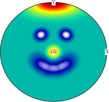

Notice the two eyes and the curved mouth in the upper hemisphere. The plot is a representation sampled densely enough to look continuous. The function itself is not a grid of stored values.

Evaluate selected directions

An S2Fun can be evaluated at any direction, whether or not that direction appeared in a plot. Here eval returns one value for each Cartesian axis.

directions = [vector3d.X,vector3d.Y,vector3d.Z];
values = eval(sF,directions)

values =
    0.0000
    0.5000
    0.3998

This distinction matters in later calculations. An extremum search or an integral acts on the spherical function rather than on the pixels of its current display.

Several representations, one interface

There is more than one way to store a function on a sphere. The choices are genuinely different rather than a matter of taste.

A harmonic representation keeps coefficients in the spherical harmonic basis, the sphere's equivalent of a Fourier series. It is exact for smooth functions, makes rotation and convolution cheap, and needs many coefficients for sharp features. A kernel or radial representation stores a sum of bumps at chosen positions. This is the natural fit for a density estimated from scattered measurements. A triangulated representation stores values at nodes and interpolates between them. It handles data that are neither smooth nor bump-like.

MTEX puts these representations behind one interface. A function can be built one way and used another without the calling code knowing which representation is stored. Representation still affects cost and sharpness. A poor choice appears as a slow computation or a peak that will not stay sharp.

class(sF)

ans =
    'S2FunHarmonic'

The smiley is stored as an S2FunHarmonic, yet the same plot and eval calls also work for the other representations. The Concept page compares their MTEX classes and their strengths in more detail.

Bandwidth is the parameter that matters

A harmonic representation ends at a finite bandwidth. This is the highest harmonic degree retained. It determines both the finest detail that can be represented and the cost of harmonic calculations.

Too low a bandwidth smears sharp peaks and creates ringing around them. Too high a bandwidth can faithfully reproduce noise. The next plot truncates a copy of the smiley while leaving the original unchanged.

sFLow = sF;
sFLow.bandwidth = 8;

newMtexFigure('layout',[1,2]);
plot(sF,'upper')
mtexTitle(['bandwidth ' num2str(sF.bandwidth)])
nextAxis
plot(sFLow,'upper')
mtexTitle(['bandwidth ' num2str(sFLow.bandwidth)])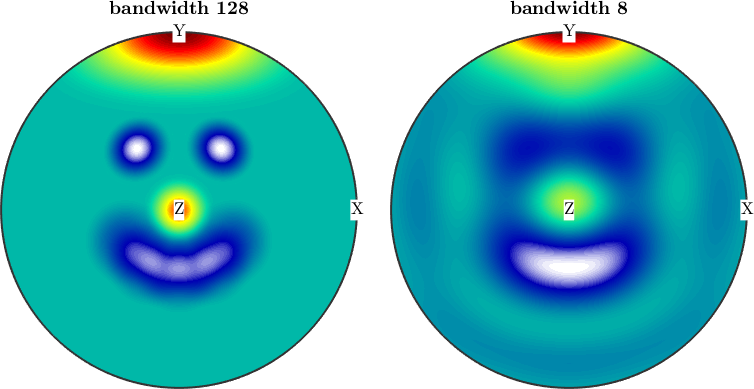

The low-bandwidth plot retains the broad layout of the face but rounds its narrow features. Oscillations also appear beside sharp transitions. Raising bandwidth improves angular detail at the cost of more coefficients.

This is the same trade-off as the halfwidth in density estimation, seen from the other side. It recurs for functions on rotations in Orientation Functions. The earlier Quadrature page explains how bandwidth controls the coefficients computed from a callable function.

Where to start

Concept surveys the representations above. Operations covers sums, products, integrals, rotations, minima, and maxima. Plotting explains the ways to draw a sphere on a page.

Getting a function from data is covered by Approximation and Interpolation. Going the other way, choosing where to evaluate it, is covered by Sampling. Sampling matters whenever an integral must be computed from a finite number of evaluations.

Spherical Harmonics and Harmonic Representation develop the basis and bandwidth used above. Spherical Kernel Functions covers the bumps in a kernel representation. Convolution explains the smoothing operation used in density estimation.

Symmetric Function handles functions that are invariant under symmetry, as a function of crystal directions must be. Bingham Distribution introduces a specific statistical model for directions.

Radon Transform turns an orientation density into a pole figure. It is therefore the mathematical heart of pole figure inversion.

Functions whose values are not numbers have their own pages: Vector Valued Spherical Functions, Vector Field, and Axis Field. The last describes fields of axes, where direction has no sign, exactly as in Vectors.

Fourier Series is the one-dimensional relative for functions of a single angle. The corresponding objects for functions on rotations are introduced in Orientation Functions. Their most important texture-analysis example is the ODF.

close all

References

Next

Continue with Concept to compare the concrete MTEX representations that share the S2Fun interface.