Quadrature of Spherical Functions

Quadrature replaces an integral over the sphere by a weighted sum at selected directions. MTEX uses those sums to compute the spherical harmonic coefficients of a function that can be evaluated at arbitrary directions. The result is an S2FunHarmonic that can be evaluated, plotted, and combined with other spherical functions.

plottingConvention.default('y↑→x');
close all

Construct a harmonic representation

Consider the scalar function \(f(\mathbf{v})=v_xv_y\). A MATLAB function handle expresses this rule for one or many vector3d directions.

fun = @(v) v.x .* v.y;

S2FunHarmonic.quadrature evaluates the handle on a quadrature grid and applies the corresponding weights. The 'bandwidth' is the largest harmonic degree retained in the result. Because this example is a quadratic polynomial, degree 2 is sufficient.

sF = S2FunHarmonic.quadrature(fun,'bandwidth',2)

sF = S2FunHarmonic (y↑→x)
  bandwidth: 2
  antipodal: true

The surface radius and colour both show the function value.

surf(sF)
mtexColorbar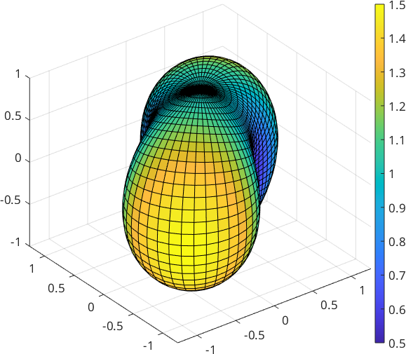

Notice the four alternating lobes around the equator. The function is zero whenever either \(v_x\) or \(v_y\) is zero, and it changes sign across each of those two great circles.

Check the recovered function

Quadrature constructs coefficients rather than merely storing the sampled values. We can therefore evaluate the result at directions that were not chosen as quadrature nodes. The maximum error below tests a regular grid with a spacing of \(5\) degrees.

vTest = reshape(regularS2Grid('resolution',5*degree),[],1);
maxError = max(abs(eval(sF,vTest) - fun(vTest)))

maxError =
   6.6613e-16

The error is at numerical round-off because the requested bandwidth contains every harmonic degree in this polynomial. For a general function, increase the bandwidth until the features or derived quantities of interest no longer change appreciably.

What bandwidth leaves out

Bandwidth 1 cannot represent the degree-2 variation of this example. The corresponding result is nearly zero, so its error remains large even though the quadrature itself has been carried out correctly.

sFLow = S2FunHarmonic.quadrature(fun,'bandwidth',1);
lowBandwidthError = max(abs(eval(sFLow,vTest) - fun(vTest)))

lowBandwidthError =
    0.6667

This is truncation error, not evidence that more scattered data are needed. Quadrature assumes a callable function over the whole sphere. If only scattered directions and values are available, use interpolation or approximation instead.

Supplying a quadrature grid explicitly

The high-level call creates its own nodes and weights. The same operation can start from an explicit quadratureS2Grid when the function values have already been evaluated there.

S2G = quadratureS2Grid(2);
values = fun(S2G);
sFGrid = S2FunHarmonic.quadrature(S2G,values);
gridResultDifference = max(abs(eval(sFGrid,vTest) - eval(sF,vTest)))

gridResultDifference =
     0

The grid carries its own weights, and the difference is at numerical round-off. Arbitrary scattered directions are not automatically a quadrature rule: their weights must represent area on the sphere. Without suitable weights, dense regions would contribute too much to the coefficients.

The maths behind quadrature

Let \(Y_n^k\) be an orthonormal spherical harmonic. Its coefficient in a function \(f\) is

\[ \hat f_n^k = \int_{S^2} f(\mathbf{v})\, \overline{Y_n^k(\mathbf{v})}\,\mathrm{d}\mathbf{v}. \]

A quadrature grid supplies nodes \(\mathbf{v}_m\) and area weights \(w_m\). MTEX approximates every coefficient through degree \(N\) by

\[ \hat f_n^k \approx \sum_m w_m f(\mathbf{v}_m) \overline{Y_n^k(\mathbf{v}_m)}, \qquad 0\leq n\leq N. \]

The 'bandwidth' option sets \(N\). It controls both the finest variation retained in the harmonic representation and the quadrature grid required to compute its coefficients.

References

Next

Continue with Harmonic Representation to inspect and truncate the coefficients produced by quadrature. If your starting point is scattered measurements, see Approximation and Interpolation.