Vectors

Directions occur throughout texture analysis. A lattice-plane normal, the rolling direction of a sheet, and the direction of a diffracted beam all answer "which way?" A force or a displacement also has a length, so it is a vector rather than only a direction.

MTEX represents both with vector3d. One variable can hold a whole list, and MTEX operations act on that list without a loop. When only direction matters, normalization divides out the length. Each unit direction is then a point on the sphere.

This page assumes basic MATLAB lists and indexing. Read Lists and Indexing if those are new. The angle and plotting conventions used throughout MTEX are collected in Notation and Conventions.

plottingConvention.default('y↑→x');

% one hundred random directions and the three Cartesian basis directions
v = vector3d.rand(100)

plot(v,'upper','grid','MarkerSize',4);
hold on;
plot([vector3d.X,vector3d.Y,vector3d.Z],...
  'labeled','backgroundColor','w');
hold off;

v = vector3d (y↑→x)
 size: 100 × 1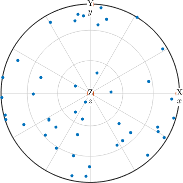

The summary reports a 100 by 1 vector3d array. This is the first point to notice: one MTEX variable stores the whole list.

In the upper-hemisphere spherical plot, X lies at the right rim, Y at the top rim, and Z at the centre. The plotting convention states that layout; it changes the drawing, not the directions. The random points on the lower hemisphere are hidden. Their stored lengths would not affect their positions in this plot. Spherical Projections explains how the sphere is mapped to the circular page.

Directions, Reference Frames, and Plots

A reference frame is the coordinate system in which data are expressed. It has an identity, a basis, and a default convention for drawing it. The random directions above are frame-free, so they use the session default when rendered. Data tied to a specimen or crystal frame use the convention carried by that frame. Axes Alignment develops reference frames, plotting conventions, and frame changes.

A spherical plot uses direction only. Use norm when length is part of the quantity, and normalize when it is not. Do not infer a vector's length from a marker's distance from the centre of a spherical plot.

Directions and Axes Are Not the Same

A direction distinguishes its two ends: north is not south. An axis does not. The axis of a twofold rotation is one example. Conventional pole figures usually treat a plane normal as an axis because Friedel's law makes opposite reflection intensities equal under its stated conditions.

MTEX records this distinction with the antipodal property. It changes calculations as well as plots. The angle between two axes is never obtuse, an axial mean does not let opposite endpoints cancel, and an axial density satisfies \(f(v)=f(-v)\).

The plot option 'upper' only hides the lower hemisphere. It does not set antipodal or identify a direction with its negative. Forgetting that distinction can produce a plausible result without an error message. Axes and Antipodal Symmetry treats the consequences in detail.

Follow the Chapter

Definition constructs vectors from Cartesian components, spherical angles, and the specimen basis directions. It also explains how to inspect components, angles, and lengths.

Import and Export exchange lists with text files. Read them after the definition when data exchange is your immediate task.

Operations covers angles, dot and cross products, rotations, projections, normalization, and vectorized list operations. Read Axes and Antipodal Symmetry before analysing data whose two signs are physically equivalent.

Density Estimation turns a measured list into a smooth function on the sphere. Spherical Grids instead constructs finite sets of directions for sampling, integration, or numerical representation.

How Vectors Connect to MTEX

Directions attached to a crystal lattice carry crystal symmetry and are written as Miller indices. They are introduced in Crystal Geometry. Rotations act on vectors without changing their lengths. Spherical Functions attach a value to every direction rather than storing a finite list of points.

The worked Tutorials use these foundations inside larger analyses. EBSD orientations map crystal directions into specimen directions, pole figures place diffraction intensity over specimen directions, and ODF calculations connect the two through orientations.

Further Reading

Next

Begin with Defining Three-Dimensional Vectors. Readers who already construct vectors comfortably can continue with Vector Operations or go directly to Axes and Antipodal Symmetry for unoriented data.