Notation and Conventions

Texture analysis depends on choices about angles, frames, axes, and units. Two correct calculations can look different when those choices differ. This page states the conventions that MTEX uses and shows how to diagnose the most common mismatches.

Use Glossary when a term itself is unfamiliar. The toolbox habits for lists, indexing, and options are in General Concepts.

plottingConvention.default('y↑→x');

Angles are radians, and degree converts them

Every angle in MTEX is in radians. There is no option to change this, and MTEX does not detect whether an input was intended to be in degrees. Multiply a value by degree when the value is stated in degrees.

10*degree

ans =
    0.1745

The result is approximately 0.1745 radians. A bare 10 passed where an angle is expected is still valid: it means 10 radians, or a little more than one and a half turns. This mistake therefore produces results that are wildly rather than subtly wrong.

Euler angles follow the Bunge convention

Three Euler angles need both an axis sequence and a rotation order. MTEX uses the Bunge convention by default: rotate about Z, then about the new X, and finally about the new Z. The angles are written phi1, Phi, phi2.

cs = crystalSymmetry('m-3m');
ori = orientation.byEuler(30*degree,50*degree,10*degree,cs);

round(Euler(ori,'Bunge')./degree)

ans =
    30    50    10

The recovered angles are 30, 50, and 10 degrees. MTEX also supports other Euler conventions, so angles from another program are unlabelled data until their convention is known.

MTEX vs. Bunge Convention explains how the MTEX coordinate map relates to the textbook statement of Bunge's convention. That comparison is not the same as selecting the Euler convention itself.

An orientation maps crystal coordinates to specimen coordinates

An orientation describes how a crystal is placed in the specimen. In MTEX, applying an orientation to a crystal direction returns the corresponding specimen direction.

h = Miller(0,0,1,cs,'uvw');   % a direction in the crystal
r = ori * h                   % where it points in the specimen

r = vector3d (y↑→x)
      x      y      z
  0.383 -0.663  0.643

Thus ori * h asks where crystal direction h points. Conversely, inv(ori) * r asks which crystal direction points along specimen direction r.

hBack = inv(ori) * r

hBack = Miller (m3̅m)
  h k l
  0 0 1

A pole figure uses the first map, while an inverse pole figure uses the second. The active and passive readings of a rotation are also inverses: one turns an object, and the other changes the axes used to describe it. See Coordinate Transformation for the full construction.

The picture makes the direction of the map visible. The translucent cube is the crystal where ori places it. The black arrows are the specimen axes, and the red arrow is crystal direction h in specimen coordinates.

cS = crystalShape.cube(cs);

figure;
plot(ori * cS,'faceAlpha',0.35,'faceColor',[0.6 0.75 0.9]);
hold on;
arrow3d(0.75*normalize(r),'faceColor','red');
arrow3d(0.75*[vector3d.X,vector3d.Y,vector3d.Z],...
  'faceColor','black');
hold off;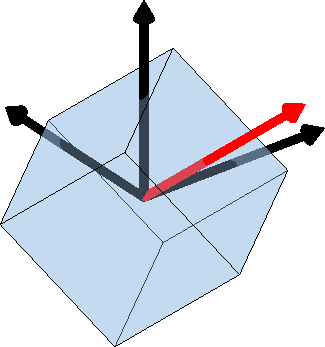

Notice that the red direction is fixed in the crystal rather than in the specimen axes. Replacing ori by inv(ori) would answer a different coordinate question and place the arrow elsewhere.

Planes and directions are different objects

Miller(1,0,0,cs) is a plane by default and uses Miller indices \((hkl)\). Add 'uvw' to construct a direction \([uvw]\). Planes and directions coincide in a cubic lattice, which makes cubic crystals a poor test of whether the correct object was constructed.

csQuartz = crystalSymmetry('321',[4.9 4.9 5.4],...
  'mineral','Quartz');

plane = Miller(1,0,0,csQuartz);
direction = Miller(1,0,0,csQuartz,'uvw');
angle(plane,direction) ./ degree

ans =
   30.0000

The \((100)\) plane normal and the \([100]\) direction are 30 degrees apart in quartz. For trigonal and hexagonal lattices, MTEX displays four indices \((hkil)\). The third index is redundant and equals \(-(h+k)\).

Crystal axes need a Cartesian alignment

A point group states which symmetry operations leave an object unchanged. It does not state how the crystallographic axes lie in a Cartesian crystal frame. For any crystal less symmetric than cubic, this alignment is a genuine choice.

The MTEX default is X||a* and Z||c. A phase may specify a different alignment when its crystal symmetry is constructed. This is why two correctly published tensors for one mineral can have different components. It also explains why data from two vendors can differ by a rotation that represents no physical change. See Crystal Axes Alignment for the available choices.

The plotting convention controls the screen axes

A plotting convention states which specimen direction points east on the page and which points out of the screen. It belongs to a reference frame, not to the measured values. A reference frame is the coordinate system in which those values are expressed.

A convention can be supplied to one plot, set for the session, or carried by the frame in which the data live.

plot(x,'how2plot','y↑→x')         % this plot only
plottingConvention.default('y↑→x') % the whole session

A copied script can therefore produce a mirrored or rotated figure when the two sessions use different defaults. Documentation pages set the convention explicitly for this reason. See Axes Alignment for frame indicators and plot options.

Units are carried by the user, not by MTEX

MTEX does not track physical units. Map lengths use the unit stored by the source file, normally micrometres. Derived values inherit that choice silently, so an area is measured in the squared map unit.

Formulas that divide one physical quantity by another need special care. Elastic stiffness is conventionally supplied in GPa and density in g/cm^3. Wave Velocities are in km/s only when those two input conventions are followed. A stiffness tensor without a density produces a number that is not a velocity at all.

ODF values are multiples of a random distribution. They are therefore dimensionless.

Names used in the examples

MTEX documentation uses the following variable names consistently. Following them makes scripts easier to compare with the examples.

Diagnose a surprising result

First check for a missing degree when a numerical result is far from the expected range. Check the Euler convention when imported triples describe the wrong orientations. Check the direction of the orientation map when a result looks like the inverse of the expected one.

For a rotated or mirrored plot, compare the plotting conventions. For a fixed rotation between two data sources, compare their crystal-frame alignments. Finally, test planes and directions in a non-cubic crystal so that an accidental interchange cannot hide behind cubic symmetry.

References

Next

Density Estimation applies these conventions when turning discrete measurements into a smooth distribution. It introduces the kernel and halfwidth that control what detail the estimate retains.

References

- H.-J. Bunge, Texture Analysis in Materials Science: Mathematical Methods, Butterworths, 1982, defines the Euler-angle convention and the orientation maps used in classical texture analysis.