General Concepts

A few habits recur in almost every MTEX analysis. The first is to think of a variable as holding many things, not one. MTEX operations usually act on the complete collection at once.

The usual workflow is short. First calculate one value per element and compare those values with a condition. The result is a logical mask: one true or false value per element. Use that mask to select the elements of interest without changing their class.

Work with collections

In MATLAB, a variable is a name for stored data. Its class determines which operations are available. An MTEX variable can contain one object or many objects of the same class.

For example, a vector3d variable may hold one direction or a list of directions. An EBSD variable represents a scan as a list of measurements. An grain2d variable may contain every grain in a map or a selected subset.

Most elementwise operations apply to the complete list. They return one result per element. This is called vectorization. It usually makes an explicit loop unnecessary and is much faster than processing elements one by one.

plottingConvention.default('y↑→x');

% one variable, five hundred directions
v = vector3d.rand(500);

% one condition, applied to all directions at once
isSteep = angle(v,vector3d.Z) < 30*degree;

plot(v(~isSteep),'upper','grid','MarkerSize',4, ...
  'MarkerFaceColor','gray')
hold on
plot(v(isSteep),'upper','MarkerSize',5,'MarkerFaceColor','red')
hold off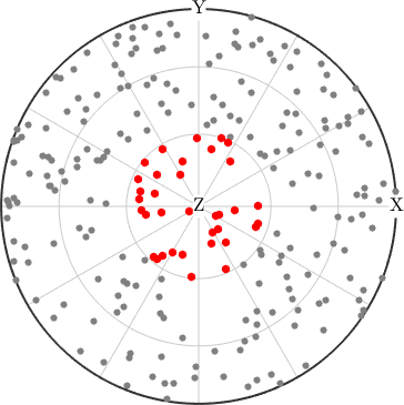

Read the selection

The red directions lie within 30 degrees of the positive \(z\) axis. The gray directions shown in the upper hemisphere lie outside that angular cap.

No loop appears in the calculation. angle compares all five hundred directions with vector3d.Z. The comparison returns one true or false value per direction. The expression v(isSteep) keeps the true entries. It returns another vector3d list, so any later vector operation accepts it.

The same two steps select grains above a chosen size, pixels of one phase, or boundaries above a chosen misorientation angle. Lists and Indexing develops this pattern with positional and logical selections.

Control one command with optional inputs

Most MTEX commands take required arguments followed by optional inputs. A flag is a bare word such as 'silent', 'antipodal', or 'contourf'. An option is a name followed by a value. For example, 'halfwidth',10*degree sets a smoothing halfwidth of 10 degrees. Flags and options may be given in any order after the required arguments.

If an option name appears twice, the last value wins and MTEX reports no error. A program that appends a default argument at the end can therefore override a value that its caller supplied.

A misspelt option name is also silently ignored. The command then uses its default and can produce a plausible result. Copy option names from the command's documentation rather than typing them from memory. Options gives a worked example and shows how to find the names a command accepts.

Do not confuse command options with stored scan options

MTEX also uses the word option for whole-scan data stored in ebsd.opt. This scan option is not an optional input to a command. The distinction from a property is determined by how many values the data contains.

A property has one value per list element. For an EBSD map, per-pixel data such as mad belongs in ebsd.prop. MTEX subsets it in lockstep with the map. Grain orientation spread, GOS, likewise has one value per grain.

A scan option describes the complete EBSD object. It does not have one value per measurement point. An imported file header containing instrument and acquisition settings is one example. Scan options remain unchanged when ebsd(ind) selects part of the map.

Putting scan-level information in prop creates a length mismatch when the map is subset. Properties shows how to inspect, add, select, and plot per-element data.

Follow the chapter in order

MTEX Scripts starts with a complete import, inspection, grain reconstruction, and plotting sequence. Lists and Indexing then explains the collection operations used in that sequence.

Configuration distinguishes a setting for one session from an option for one command. It also explains persistent defaults for fonts, figure sizes, and plotting conventions. Options gives the full account of flags and options. Properties covers per-element and whole-scan data.

Two pages are intended mainly for lookup. Glossary defines vocabulary used across the documentation. It places easily confused terms side by side. These include misorientation and disorientation, halfwidth and bandwidth, and hole and inclusion. Notation and Conventions records choices that affect results. These include radians, Bunge Euler angles, the direction in which an orientation acts, planes versus directions, and crystal-axis alignment. Consult it first when a figure is mirrored or a number differs by an unexplained factor.

The final pages introduce ways to summarize a population. Density Estimation turns discrete measurements into a smooth distribution. Optimal Kernel explains how to choose the amount of smoothing. This is the recurring halfwidth question in MTEX density estimates. Clustering instead groups nearby orientations without fitting a density.

After these foundations, Tutorials is the fastest route into a complete application. Plotting explains how MTEX figures are assembled. Vectors begins the reference material for the basic object types.

References

This overview documents MTEX collection and calling conventions. It does not rely on an external method or definition.

Next

Continue with MTEX Scripts to build and inspect a short, reproducible analysis from import through grain-boundary plotting.