Defining Three-Dimensional Vectors

A vector3d stores one or more vectors through their Cartesian components \(x\), \(y\) and \(z\). A reference frame identifies the coordinate system in which data are expressed. It includes an identity, basis and default plotting convention. The components are coordinates in that frame.

A vector also has a length. When only its direction matters, dividing out that length gives a point on the unit sphere. This spherical view underlies specimen directions, pole figures and crystal directions throughout MTEX. Crystal directions add lattice information and are introduced in Miller Indices.

This page assumes basic MATLAB arrays and indexing. See Lists and Indexing if those are new to you.

plottingConvention.default('y↑→x');

Cartesian Coordinates

Define a vector directly from its three Cartesian components.

v = vector3d(1,2,3)

v = vector3d (y↑→x)
  x y z
  1 2 3

The summary reports one vector and lists its \(x\), \(y\) and \(z\) components. A spherical plot uses its direction and therefore divides out its length.

plot(v,'grid','upper');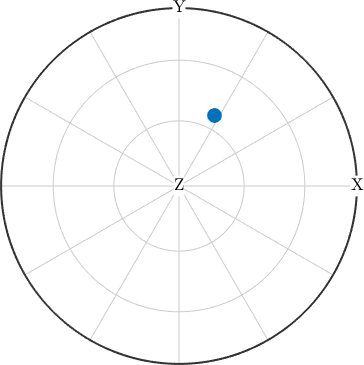

The point lies in the upper-right quadrant because \(x\) and \(y\) are positive. It lies inside the rim because \(z\) is positive. Multiplying all three components by the same positive number would not move this point. Spherical Projections explains how the sphere is mapped onto the page.

The norm is the stored vector's length.

norm(v)

ans =
    3.7417

For \((1,2,3)\) the result is \(\sqrt{14}\), displayed here as 3.7417. normalize divides each component by that length, so the result has length one without changing direction.

norm(normalize(v))

ans =
     1

A zero vector has no direction, so its normalized components are undefined.

normalize(vector3d(0,0,0))

ans = vector3d (y↑→x)
    x   y   z
  NaN NaN NaN

The output contains three NaN values. Check for zero length before normalizing measured data.

Individual coordinates can be read and changed as properties.

v.x

ans =
     1

v.x = 0

v = vector3d (y↑→x)
  x y z
  0 2 3

The displayed row is now \((0,2,3)\). Changing a component preserves neither the previous length nor the previous direction.

Polar Coordinates

A direction can also be described by two angles. The polar angle \(\theta\) is measured away from the Z axis. The azimuth angle \(\rho\) is measured in the XY plane away from the X axis. vector3d.byPolar takes the angles in that order and returns a unit vector.

v = vector3d.byPolar(60*degree,45*degree)

v = vector3d (y↑→x)
      x     y     z
  0.612 0.612   0.5

MTEX stores angles in radians. Multiplying by degree converts a value in degrees to radians for input.

plot(v,'grid','upper');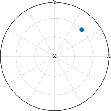

The point is \(60^\circ\) from Z and turns \(45^\circ\) from X towards Y. Thus \(\theta\) controls its distance from the centre of this spherical plot, while \(\rho\) controls the direction around the centre.

The angle properties read back in radians. Divide by degree to display them in degrees.

v.rho ./ degree   % azimuth angle in degrees

ans =
   45.0000

v.theta ./ degree % polar angle in degrees

ans =
   60.0000

Basis Directions and Reference Frames

The constants vector3d.X, vector3d.Y and vector3d.Z spell the three Cartesian basis directions. They make combinations easier to read.

v = vector3d.X + 2*vector3d.Y

v = vector3d (y↑→x)
  x y z
  1 2 0

The summary shows the components \((1,2,0)\). Fresh vector3d data are frame-free. They are not tied to a named measurement, rolling or geological frame. At plotting time they follow the session's default specimen frame. Axes Alignment explains named frames and their plotting conventions.

Many Directions at Once

One vector3d variable can hold a whole array of vectors. MTEX operations act on the array at once, so loops over individual vectors are usually unnecessary. Passing coordinate arrays creates one vector per entry.

v = vector3d(1:5,0,1)

v = vector3d (y↑→x)
 size: 1 × 5
  x y z
  1 0 1
  2 0 1
  3 0 1
  4 0 1
  5 0 1

The displayed summary contains five rows. The array has a shape and uses the same indexing rules as a numeric MATLAB array.

size(v)

ans =
     1     5

v(2)

ans = vector3d (y↑→x)
  x y z
  2 0 1

The second row, \((2,0,1)\), is returned as another vector3d object. When coordinates are already arranged in a matrix, vector3d.byXYZ reads one vector from each row.

xyz = [1 0 0; 0 1 0; 1 1 1];
v = vector3d.byXYZ(xyz)

v = vector3d (y↑→x)
 size: 3 × 1
  x y z
  1 0 0
  0 1 0
  1 1 1

The three output rows match the three matrix rows. Prefer byXYZ when the row convention matters. The constructor also accepts coordinate matrices. A \(3 \times 3\) matrix could mean vectors by rows or by columns, so the constructor warns about that ambiguity and reads by columns.

vector3d.rand creates uniformly distributed random unit directions. The following call creates 100 directions. Its long object summary is not useful here, so the semicolon keeps it out of the page.

v = vector3d.rand(100);

plot(v,'upper','grid','MarkerSize',4);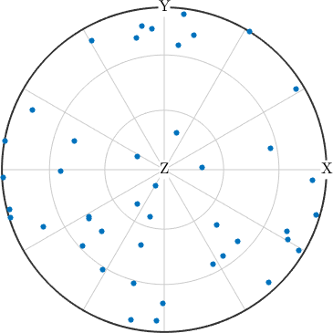

The plot handles the complete array in one call. Only directions on the upper hemisphere appear because of 'upper'; the option does not identify a direction with its negative.

Plotting Conventions

A plotting convention states how a reference frame is laid out on screen. It does not change the vector or re-express it in another frame. Pass 'how2plot' to change one plot.

v = vector3d(1,2,3);

plot(v,'how2plot','z←↑y','grid');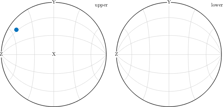

The axis annotation now shows Z pointing left and Y pointing up. The components and length of v have not changed. To align subsequent plots, use the explicit string form of plottingConvention.default shown at the start of this page. Axes Alignment develops frame changes and plotting conventions in full.

Directions and Axes

A direction distinguishes its two ends, so v and -v point in different directions. An axis treats those two signs as equivalent. The 'upper' option only selects a hemisphere. It does not turn a direction into an axis. Axes and Antipodal Symmetry explains how the antipodal flag changes angles, means and densities.

Further Reading

Next

Operations develops angles, dot and cross products, normalization and means over arrays. Read Axes and Antipodal Symmetry next. It explains how to treat plane normals and conventional diffraction poles as axes.