Pole Figures

Diffraction pole figures describe crystallographic texture without locating individual crystals. A pole figure is the distribution of normals to one family of lattice planes over directions in the specimen reference frame.

An X-ray or neutron experiment first records diffraction intensity. After background and defocusing corrections and normalization, that intensity is a quantitative pole density. Keeping these two stages separate prevents raw counts from being mistaken for multiples of a random distribution (mrd).

Diffraction averages all illuminated crystals at once. It can probe a bulk volume without a vacuum or a conductive sample, and it often counts many more crystals than an orientation map. The price is spatial information: a pole figure says which orientations occur, not where they occur.

This chapter assumes the Miller-index notation introduced in Miller Indices. Before reconstructing an orientation distribution function (ODF), review its definition and units in ODF Theory.

plottingConvention.default('y↑→x');
mtexdata dubna silent

pf

pf = PoleFigure (y↑→x)
  crystal symmetry : Quartz (321, X||a*, Y||b, Z||c)
 
  h = (022̅1), r = 72 × 19 points
  h = (101̅0), r = 72 × 19 points
  h = (101̅1)(011̅1), r = 72 × 19 points
  h = (101̅2), r = 72 × 19 points
  h = (112̅0), r = 72 × 19 points
  h = (112̅1), r = 72 × 19 points
  h = (112̅2), r = 72 × 19 points

The summary lists seven measured pole figures from one quartz specimen. One entry contains two lattice planes because their diffraction peaks were too close to separate. Its intensity is the weighted sum of both pole figures, so the reconstruction must include both planes and their coefficients rather than treating the entry as a single reflection.

The plotting convention draws specimen Y upwards and specimen X to the right. It changes the screen layout, not the specimen reference frame or the measured directions.

plot(pf,'figSize','small')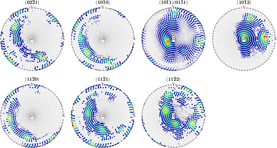

Notice that the bands and maxima occupy different specimen directions in different panels. Each lattice-plane family therefore supplies a different projection of the same texture, and the projections constrain one another. Superposed reflections are common measurements rather than errors; the two-plane title identifies the one in this data set.

What one pole-figure value means

An ODF is a density over the three-dimensional space of orientations. For a lattice-plane normal \(h\) and a specimen direction \(r\), one pole-figure value sums the ODF over every orientation that maps \(h\) onto \(r\).

Those orientations form a one-dimensional fibre in orientation space. The integral along that fibre is the pole-figure transform of the ODF, also called its Radon transform. Pole Figures of an ODF develops this forward projection, while The Spherical Radon Transform introduces the underlying operation on the sphere.

A pole figure is therefore a two-dimensional projection of a three-dimensional distribution. Measuring several lattice-plane families reduces the ambiguity caused by having too few projections, but the inverse problem still does not have a unique answer.

What ordinary diffraction cannot determine

Under Friedel's law, ordinary diffraction cannot distinguish the two sides of a lattice plane. Its pole figures are antipodally symmetric even when the material's orientation distribution is not. In a harmonic expansion, the measurements determine the even-degree terms of the ODF but not the odd-degree terms.

Anomalous-scattering experiments can break this equivalence, but additional conventional pole figures cannot. This is a different limitation from measuring too few lattice-plane families, so the two should not be confused.

A reconstruction must choose the missing odd part by an assumption. Different choices can weaken real components, raise the uniform background, or create spurious peaks where the material has none. These inversion artefacts are called ghosts.

Ghost correction makes that choice more defensible, but it does not turn an assumption into measured information. A close match between measured and recalculated pole figures is necessary validation; it is not proof that the reconstructed ODF is unique or correct.

Recommended reading order

Start with Import and Plot to bring measured data into MTEX and inspect it. Continue with Modify for background subtraction, defocusing, normalization, incomplete coverage, outliers, and justified rotations.

ODF Reconstruction develops the direct inversion, and Iterative ODF Reconstruction changes its representation scale or measurement density. The latter assumes the direct workflow and cannot remove its non-uniqueness.

Simulation then runs the forward and inverse problems with a known ODF. It also assumes ODF Modelling and Pole Figures of an ODF. This controlled experiment is the most reliable way to see what a reconstruction preserves.

Next read The Ghost Effect and Ghost Correction. They separate the limitations caused by too few pole figures from information that ordinary diffraction never measured.

Santa Fe Example tests the choices on a standard model whose true ODF is known. Dubna Example applies the validation sequence to measured neutron data, where no true ODF is available. Export closes the route by exchanging measured or recalculated pole figures with other software.

Further reading

Next

A reconstructed ODF can be explored with ODF Analysis. In the main documentation route that chapter supplies the theory used here; the next measurement chapter is EBSD Analysis. EBSD assigns orientations point by point on a polished surface and retains the spatial information that a bulk diffraction pole figure averages away.

Spherical Functions and Orientation Functions develop the mathematical function spaces behind pole figures and ODFs.