Regular ODF estimation
Please refer to PoleFigure2ODF tutorial first. The regular way of estimating an ODF:
mtexdata dubna
odf_naive = calcODF(pf);

calcError(pf,odf_naive)
pf = PoleFigure (y↑→x)
crystal symmetry : Quartz (321, X||a*, Y||b, Z||c*)
h = (02-21), r = 72 x 19 points
h = (10-10), r = 72 x 19 points
h = (10-11)(01-11), r = 72 x 19 points
h = (10-12), r = 72 x 19 points
h = (11-20), r = 72 x 19 points
h = (11-21), r = 72 x 19 points
h = (11-22), r = 72 x 19 points
ans =
0.4439 0.3836 0.2585 0.3508 0.3407 0.4099 0.3669visual inspection
odf_naive.plot(pf.allH)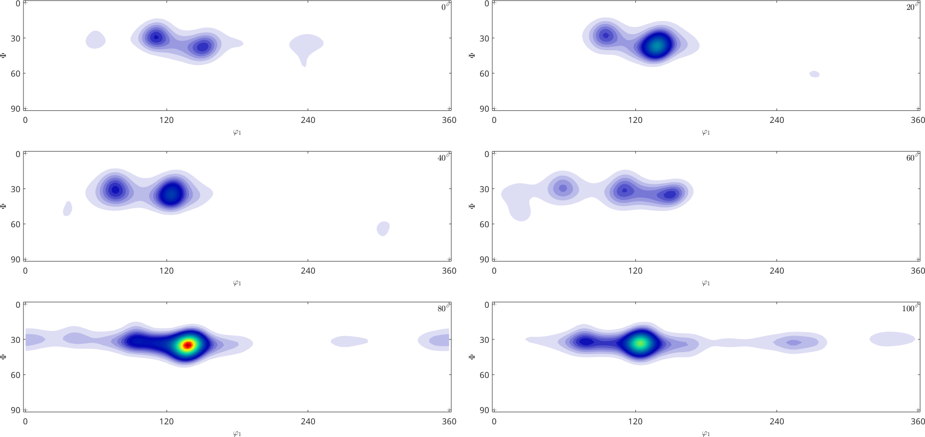
another form to regularize the inversion problem is to iteratively adjust the kernel width during ODF estimation.
odf_iter = calcODFIterative(pf,'nothinning');

calcError(pf,odf_iter)
ans =
0.3207 0.1989 0.2120 0.2095 0.1741 0.2811 0.2902visual inspection
odf_iter.plot(pf.allH)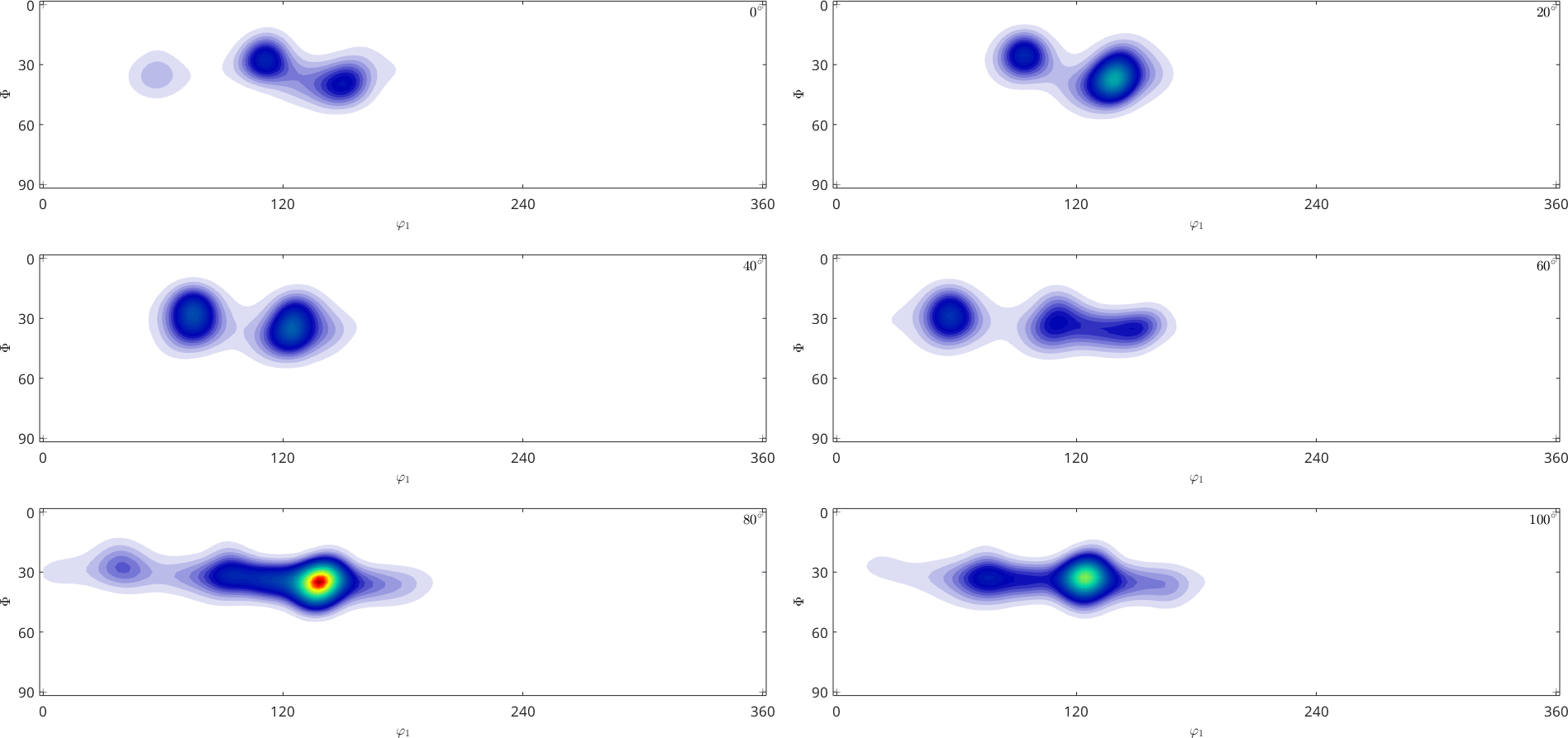
volume portion that is differently distributed between the two methods
calcError(odf_iter,odf_naive,'l1')ans =
0.2428visual inspection indicates that the uniform portion is distributed differently
plot(calcPoleFigure(pf,odf_naive-odf_iter))
%plotDiff(odf_naive,odf_iter)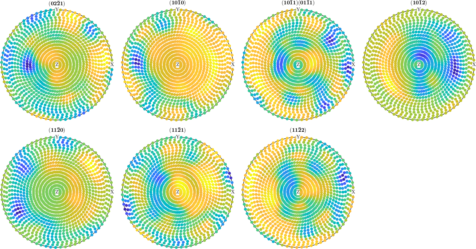
Some arbitrary modelODF of a somewhat sharp texture
demonstrated the iterative ODF estimation with a synthetic data set.
cs = crystalSymmetry('cubic');
ss = specimenSymmetry;

q = rotation.byEuler(10*degree,10*degree,10*degree,'ABG');
q2 = rotation.byEuler(10*degree,30*degree,10*degree,'ABG');

odf_true = .6*unimodalODF(q,cs,ss,'halfwidth',5*degree) + ...
            .4*unimodalODF(q2,cs,ss,'halfwidth',4*degree);
Pole Figures to measure
h = [ ...
  Miller(1,1,1,cs), ...
  Miller(1,0,0,cs), ...
  Miller(1,1,0,cs), ...
  ];

figure, odf_true.plotPDF(h)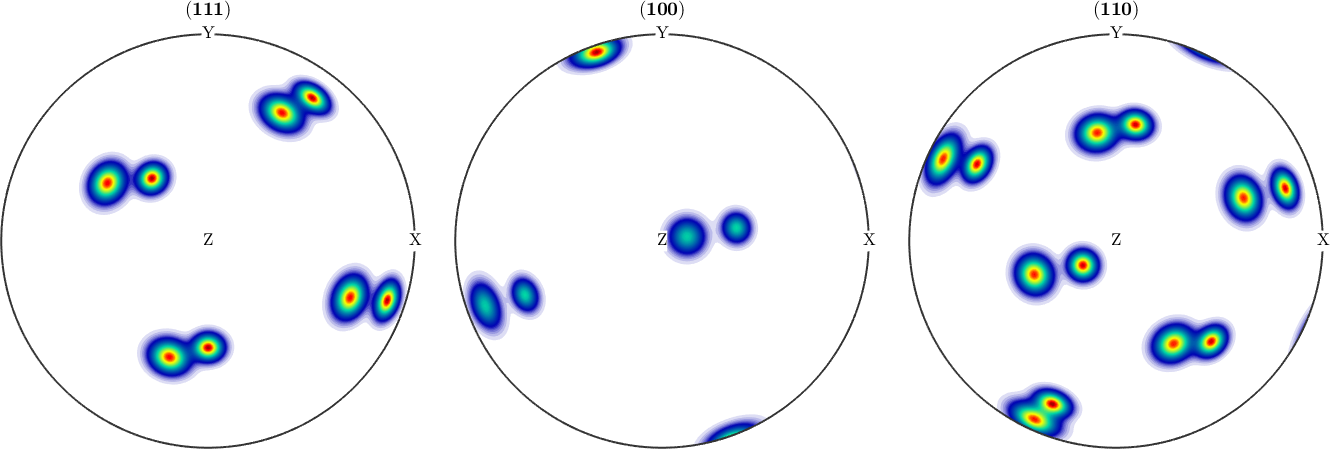
Initial measure grid
r = equispacedS2Grid('resolution',15*degree,'maxtheta',80*degree);

figure
plot(r,'markersize',12)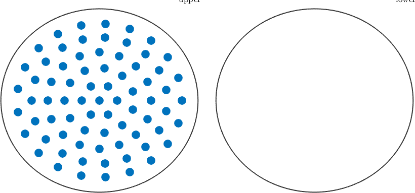
Refinement
for selected directions r we perform a 'point' like measurement.
r = equispacedS2Grid('resolution',15*degree,'maxtheta',80*degree);
r = repcell(r,size(h));
pf_measured = [];
pf_simulated = [];
pf_sim_h = {};
% number of refinement steps
nsteps = 5;

for k=1:nsteps

  % perform for every Pole Figure a measurement
  pf_simulated = calcPoleFigure(odf_true,h,r,'silent');

  % merge the new measurements with old ones
  pf_measured = union(pf_simulated,pf_measured);
  plot(pf_measured,'silent')
  drawnow

  fprintf('- at resolution : %f\n', mean(cellfun(@(r) r.resolution, pf_measured.allR))/degree);

  if k < nsteps
    % odf modeling
    odf_recalc = calcODF(pf_measured,'zeroRange','silent');

    % in order to minimize the modeling error
    pf_recalcerror  = calcErrorPF(pf_measured,odf_recalc,'l1','silent');

    % we could initialized initial weights with previous estimation
    odf_recalcerror = calcODF(pf_recalcerror,'silent');

    % the error we don't know actually
    fprintf('  error true -- estimated odf   : %f\n', calcError(odf_true,odf_recalc,'silent'))

    % refine the grid for every polefigure
    for l=1:length(h)
      r_old = pf_measured{l}.r;
      [newS2G, r_new] = refine( r_old(:) );

      % selection of points of interest, naive criterion
      pf_sim_h = calcPoleFigure(odf_recalc, h(l),  r_new,'silent');
      th = quantile(pf_sim_h.intensities,0.75);
      r{l} = pf_sim_h.r(pf_sim_h.intensities > th);
    end
  end
end
- at resolution : 14.545455
error true -- estimated odf : 0.941439
- at resolution : 13.009430
error true -- estimated odf : 0.405335
- at resolution : 9.506983
error true -- estimated odf : 0.236237
- at resolution : 6.738829
error true -- estimated odf : 0.303526
- at resolution : 3.753827
Measured Pole Figure
pf_measured
plot(pf_measured,'silent');
pf_measured = PoleFigure (y↑→x)
crystal symmetry : m-3m
h = (111), r = 367 x 1 points
h = (100), r = 367 x 1 points
h = (110), r = 367 x 1 points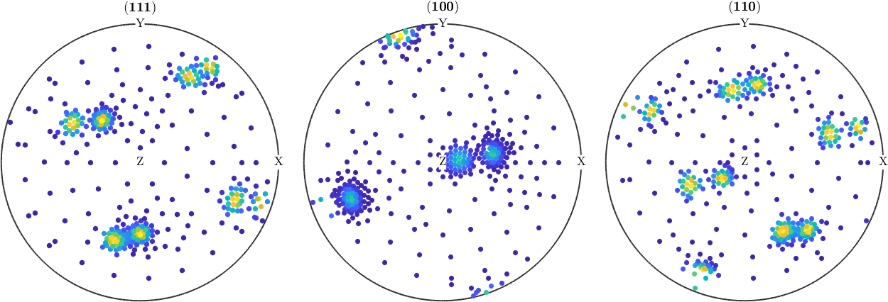
Final model
the default odf estimation will distribute volume on nodes that do not have corresponding data.
odf_recalc = calcODF(pf_measured,'zeroRange','resolution',2.5*degree);
fprintf('  error true -- estimated odf   : %f\n', calcError(odf_true,odf_recalc))
error true -- estimated odf : 0.400117Compare with iterative odf estimation
the iterative odf estimation will model the volume portions of nodes that do not have corresponding data by assuming volume portions coming from a broader halfwidth, thus the error to the true odf will be significantly smaller.
odf_recalc_iterative = calcODFIterative(pf_measured,'halfwidth',2.5*degree);
fprintf('  error true -- iter. est. odf  : %f\n', calcError(odf_true,odf_recalc_iterative))
error true -- iter. est. odf : 0.114767volume portion that is differently distributed
calcError(odf_recalc,odf_recalc_iterative,'l1')ans =
0.3167