The Tangent Space on the Rotation Group

Tangent vectors on the rotation group can be thought of as directions in which a rotation can be varied. Since these directions depend on the specific rotation you start from, they are not global but local objects. The set of all tangent vectors at a given rotation forms the tangent space, which describes the local geometry of the rotation group in the neighborhood of that point.

Definition of Tangent Spaces and Tangent Vectors on the Rotation Group

First we start with a (slightly technical) mathematical description of the tangent space by spinTensor's, which are used to describe small rotational changes. For more information take a look here in the documentation.

The tangent space of the rotation group at some rotation \(R\) has two different representations. There is a left and a right tangent space representation.

The left tangent space is defined by

\[ T_R SO(3) = \{ S \cdot R | S=-S^T \} = \mathfrak{so}(3) \cdot R, \]

where \(\mathfrak{so}(3)\) describes the set of all skew symmetric matrices, i.e. spinTensor's.

R = rotation.byAxisAngle(xvector,20*degree);
S1 = spinTensor(vector3d(0,0,1))
% left tangent vector at some Rotation R
TV = matrix(S1) * matrix(R)

S1 = spinTensor (y↑→x)
  rank: 2 (3 x 3)
 
  0 -1  0
  1  0  0
  0  0  0
TV =
            0     -0.93969      0.34202
            1            0            0
            0            0            0

The right tangent space is defined analogously:

\[ T_R SO(3) = \{ R \cdot S | S=-S^T \} = R \cdot \mathfrak{so}(3). \]

Again, skew-symmetric matrices describe all possible infinitesimal rotations, but now applied on the right side of R.

S2 = spinTensor(vector3d(0,sin(20*degree),cos(20*degree)))
% right tangent vector at some rotation R
TV = matrix(R)*matrix(S2)

S2 = spinTensor (y↑→x)
  rank: 2 (3 x 3)
 
 *10^-2
      0 -93.97   34.2
  93.97      0      0
  -34.2      0      0
TV =
            0     -0.93969      0.34202
            1            0            0
   5.5511e-17            0            0

Note that the left and right tangent spaces describe the same tangent vectors, just in different notations.

In the above example S1 and S2 describe the same tangent vector TV in different representations.

Description of Rotational Tangent Vectors in MTEX

In MTEX, tangent vectors are represented as objects of the class SO3TangentVector. Therefore the three distinguish entries of the spinTensor \(S\) are stored as vector3d, in the following way:

S = spinTensor(0.2*vector3d(1,2,3))
v1 = SO3TangentVector(S,R)

S = spinTensor (y↑→x)
  rank: 2 (3 x 3)
 
 *10^-2
   0 -60  40
  60   0 -20
 -40  20   0
 
v1 = SO3TangentVector (y↑→x)
 intern symmetries: 1 → y↑→x
 TagentSpace: leftVector
    x   y   z
  0.2 0.4 0.6

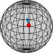
A SO3TangentVector in MTEX has three important properties:

By default, the tangent space representation is left. A right tangent vector can be constructed as follows:

v2 = SO3TangentVector(vector3d(1,2,3),R,SO3TangentSpace.rightVector)

v2 = SO3TangentVector (y↑→x)
 intern symmetries: 1 → y↑→x
 TagentSpace: rightVector
  x y z
  1 2 3

Here v1 and v2 have the same coordinates in different bases (tangent space representations). Hence they describe different tangent vectors.

Left and right tangent vectors can be easily transformed into each other:

v1_right = right(v1)
v1_left = left(v1_right)

v1_right = SO3TangentVector (y↑→x)
 intern symmetries: 1 → y↑→x
 TagentSpace: rightVector
    x        y        z
  0.2 0.581089 0.427008
 
v1_left = SO3TangentVector (y↑→x)
 intern symmetries: 1 → y↑→x
 TagentSpace: leftVector
    x   y   z
  0.2 0.4 0.6

Note that MTEX cares about the tangent space representation. Hence if we try to compute with @SO3TangentVectors MTEX automatically transform them into the same representation and applies the operation afterwards.

v1 + v1_right

ans = SO3TangentVector (y↑→x)
 intern symmetries: 1 → y↑→x
 TagentSpace: leftVector
    x   y   z
  0.4 0.8 1.2

Operations of Rotational Tangent Vectors

The following operations are defined for rotational tangent vectors TV, TV1, TV2

Exponential and Logarithm Map of Tangent Vectors

In the context of the rotation group SO(3), the exponential and logarithm maps provide the link between tangent vectors and rotations.

The exponential map takes a tangent vector (an infinitesimal rotation) and returns the corresponding finite rotation in SO(3). It is performed onto the tangent vector v1 with the command exp.

rot = exp(v1)

rot = orientation (1 → y↑→x)
 
  Bunge Euler angles in degree
     phi1     Phi    phi2
  59.1419 41.5248 332.468

The logarithm map does the reverse: It takes two rotations and computes the tangent vector in the tangent space of one rotation that points towards the other rotation. % It is performed onto the rotations with the command log.

log(rot,R)

ans = SO3TangentVector (y↑→x)
 intern symmetries: 1 → y↑→x
 TagentSpace: leftVector
    x   y   z
  0.2 0.4 0.6

Together, these maps allow switching between the curved geometry of SO(3) and the linear structure of its tangent spaces, which is essential for interpolation, averaging, and optimization on rotations.