Correcting Pseudo Symmetry

A pseudo symmetry is a rotation that is not a symmetry of the crystal, but maps its diffraction pattern almost onto itself. An indexing algorithm may therefore alternate between the true orientation and a rotated alternative. One physical crystal region then appears as several reconstructed grains, separated by the pseudo-symmetric misorientation.

This is an indexing failure, not ordinary orientation noise. It also is not proof of a physical domain or twin: a real boundary can have the same misorientation. The command cleanUpPseudoSym combines crystallography with a spatial heuristic to tell them apart.

The page assumes the grain structure has been reconstructed as described in grain reconstruction. The pages on boundary misorientations and orientation symmetry introduce the geometry used below.

A Map With Pseudo Symmetry

Olivine is a classical example. Its oxygen sublattice is almost hexagonally close packed with the stacking axis along [100]. Rotations about [100] by multiples of 60 degrees therefore map the oxygen positions nearly onto themselves, although the true symmetry mmm contains only the 180 degree rotation.

plottingConvention.default('y↑→x');
mtexdata forsterite silent

% consider only indexed data
ebsd = ebsd('indexed');

% reconstruct the grain structure
[grains,ebsd] = calcGrains(ebsd,'angle',10*degree,'minPixel',5);

% use one colour key for every orientation map on this page
ipfKey = ipfColorKey(ebsd('Fo'));
foColor = ipfKey.orientation2color(ebsd('Fo').orientations);

% plot the orientation map of the Forsterite phase
plot(ebsd('Fo'),foColor)

hold on
plot(grains.boundary,'linewidth',1.5)
hold off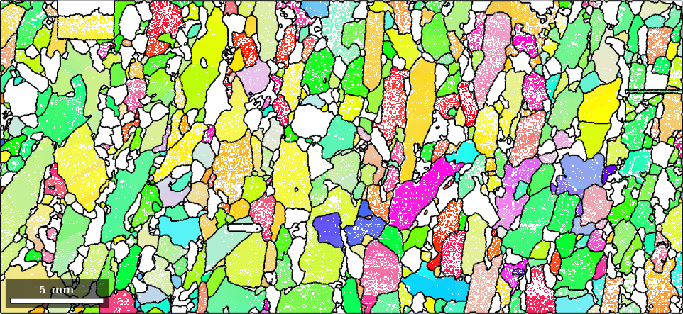

The second output of calcGrains assigns the per-measurement property ebsd.grainId. The cleanup uses it to connect every orientation with its reconstructed grain.

At this scale the pseudo symmetry is invisible. The correction at the end of this page moves 275 of the 152345 forsterite measurements, under two tenths of a percent, and it does so in patches of a few dozen pixels sitting inside much larger host grains. The rest of this page therefore finds those patches by their misorientation, and zooms into one of them once they are known.

The boundaries have deliberately not been smoothed. Since cleanUpPseudoSym decides from their raggedness, smoothing must be applied after the correction and not before.

Detecting the Pseudo Symmetry

When the pseudo symmetry is not known beforehand, look for it in the distribution of boundary misorientations. Olivine suggests a rotation near 60 degrees, so select those boundaries and plot the distribution of their rotational axes.

% misorientations at all Forsterite--Forsterite boundaries
mori = grains.boundary('Fo','Fo').misorientation;

% restrict to rotational angles close to 60 degrees
mori = mori(mori.angle > 55*degree & mori.angle < 65*degree);

% plot the distribution of rotational axes
plot(mori.axis,'contourf','fundamentalRegion','halfwidth',5*degree)
mtexColorbar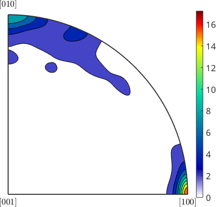

The sharp maximum at [100] establishes both parts of the candidate: a rotation of about 60 degrees around [100]. Define that operation as a misorientation with byAxisAngle.

cs = ebsd('Fo').CS;
psSym = orientation.byAxisAngle(Miller(1,0,0,cs,'uvw'),60*degree);

Modulo the true symmetry mmm, the rotations by 60 and 120 degrees are different operations. The latter is the inverse of the former, and both occur because the indexer may have chosen either solution. It is enough to pass one of them to cleanUpPseudoSym.

A measurement stores a fixed representative of an orientation. Its alternative is therefore not simply ori * psSym, but ori * s * psSym for some true symmetry element s. The command generates all these operators itself, so passing 60 degrees, 120 degrees, or both gives the same result.

The pseudo symmetry is a misorientation, so it has the same crystal symmetry on both sides. The condition psSym.CS == psSym.SS is required by cleanUpPseudoSym and tells the command which phase to correct.

Pseudo-Symmetric Grain Boundaries

Select all boundary segments whose misorientation matches the candidate. A grain boundary has no direction: its misorientation carries the grain exchange symmetry explained in grain exchange symmetry. The test therefore catches both indexing alternatives at once.

gB = grains.boundary('Fo','Fo');
gB = gB(any(angle(gB.misorientation,psSym) < 2*degree,2))

gB = grainBoundary (y↑→x)
 
 Segments   length   mineral 1   mineral 2
      143  7534 µm  Forsterite  Forsterite

% a region containing one pseudo-symmetric patch
region = [27300 1900 1000 700];

% plot the orientation map of this region
ebsdS = ebsd(inpolygon(ebsd,region));
foColor = ipfKey.orientation2color(ebsdS('Fo').orientations);
plot(ebsdS('Fo'),foColor)

% overlay all boundaries and highlight the matching ones
hold on
plot(grains.boundary,'linewidth',1.5)
plot(gB,'linewidth',3,'linecolor','r')
hold off

% the boundary overlay covers the whole map, so keep the view on the region
xlim([region(1) region(1)+region(3)]), ylim([region(2) region(2)+region(4)])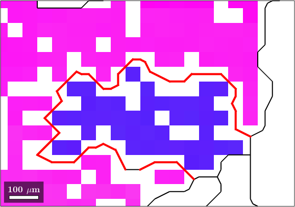

The blue patch has been indexed with the alternative solution. Its red boundary repeatedly detours around single pixels instead of following a stable interface. This is the spatial signature used by the cleanup.

Raggedness is evidence, not proof. A physical interface can be tortuous, and a large, coherently misindexed domain can have a smooth outline. Where the distinction matters, inspect the original patterns or reindex them against both candidate orientations. This post-processing step cannot recover information that the orientation map no longer contains.

The Tortuosity Criterion

The usual geometric intuition is boundary length divided by the distance between its endpoints. The implementation uses a closely related span: the diagonal of each component's axis-aligned bounding box. For boundary length \(L\) and box diagonal \(d_{\mathrm{box}}\), it computes

\[ \tau = \frac{L}{d_{\mathrm{box}}}. \]

A straight component has a value close to one, while detours increase its length without increasing its span. Because these are unsmoothed grid boundaries, even a physical straight interface has some staircase length; the threshold is therefore empirical rather than universal.

% connected components of the matching boundary segments
compId = gB.componentId;

% total length of each component
len = accumarray(compId,gB.segLength);

% diagonal of each component's axis-aligned bounding box
xmin = accumarray(compId,gB.midPoint.x,[],@min);
xmax = accumarray(compId,gB.midPoint.x,[],@max);
ymin = accumarray(compId,gB.midPoint.y,[],@min);
ymax = accumarray(compId,gB.midPoint.y,[],@max);
dist = sqrt((xmax-xmin).^2 + (ymax-ymin).^2);

% tortuosity and segment count of each component
tortuosity = len ./ dist;
numSeg = accumarray(compId,1);

% compare the components with the default threshold
plot(numSeg,tortuosity,'o','MarkerFaceColor','b')
hold on
plot(xlim,[1.5 1.5],'r--')
hold off
xlabel('number of segments'), ylabel('tortuosity')

numNonFinite = nnz(~isfinite(tortuosity));
fprintf('%d components have non-finite tortuosity\n',numNonFinite);

2 components have non-finite tortuosity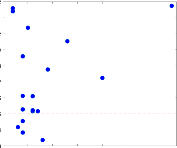

Components above the red line are candidates for correction. Very short components are unreliable: a single segment has zero box diagonal and hence infinite tortuosity. The printed count is two for this map, which is why those components do not appear at a finite height in the plot. cleanUpPseudoSym considers only components with more than four segments.

Correcting the Map

cleanUpPseudoSym merges grains separated by candidate boundaries and tests the available pseudo-symmetry operators at every affected measurement. It selects the operator closest to the mean orientation of the merged grain. The intended effect is to rotate the smaller alternative patch into the larger one, while the per-measurement test avoids assuming that every pixel in that patch chose the same representative.

The command returns the corrected EBSD data, the merged grains, and the number of measurements whose orientation changed.

[ebsdC,grainsC,numChanged] = cleanUpPseudoSym(ebsd,grains,psSym);
fprintf('%d measurements changed orientation\n',numChanged);

275 measurements changed orientation

Plot the same region again to check the correction spatially.

ebsdS = ebsdC(inpolygon(ebsdC,region));
foColor = ipfKey.orientation2color(ebsdS('Fo').orientations);
plot(ebsdS('Fo'),foColor)

hold on
plot(grainsC.boundary,'linewidth',1.5)
hold off

xlim([region(1) region(1)+region(3)]), ylim([region(2) region(2)+region(4)])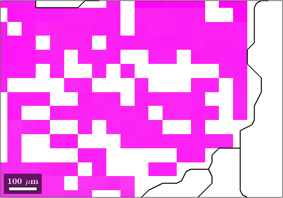

The blue alternative patch and its internal boundary have disappeared. The enclosing forsterite grain now has one consistent orientation colour, while unrelated grain boundaries remain.

Only now, with the pseudo-symmetric boundaries removed, does it make sense to smooth the grain boundaries with smoothBoundary.

grainsC = smoothBoundary(grainsC,5);

Choosing the Options

The option 'delta' is the angular tolerance within which a boundary misorientation must match the pseudo symmetry. The option 'threshold' is the minimum tortuosity for correction. Their defaults are 2 degrees and 1.5, respectively.

[ebsdC,grainsC] = cleanUpPseudoSym(ebsd,grains,psSym,...
  'delta',2*degree,'threshold',1.5);

Increasing 'delta' admits more boundary segments, while lowering 'threshold' accepts smoother components. Both changes make the cleanup more aggressive and can remove real grain boundaries. Inspect the axis distribution, the tortuosity plot, and representative regions before choosing either value.

Since the pseudo symmetry determines the corrected phase, only one phase is treated per call. To clean several phases, call the command once for each phase with that phase's pseudo symmetries.

Further Reading

Next

Grain Boundary Smoothing continues with boundary geometry after the correction. Denoising treats random orientation scatter, which is a different failure mode.