Smoothing Algorithms

Grain Boundary Smoothing introduces smoothBoundary. This page explains its three stages, the tolerances they use, and the four filters available for the last stage.

The page assumes that grains have already been reconstructed as in Grain Reconstruction. A grain boundary is one segment between neighbouring EBSD measurements that belong to different grains. A chain is a maximal run of those segments from one junction to the next. Grain Boundary Properties introduces this representation in detail.

close all;
mtexdata csl silent
[grains,ebsd] = ebsd.calcGrains('minPixel',3);

% characteristic length of the measured boundary segments
d = median(grains.boundary.segLength);

% compute the colours explicitly to keep the published output quiet
indexed = ebsd('indexed');
colorKey = ipfColorKey(indexed);
ipfColors = colorKey.orientation2color(indexed.orientations);
plot(indexed,ipfColors,'micronbar','off')
hold on
plot(grains.boundary('indexed'),'linewidth',5,'linecolor','YellowGreen')
hold off
axis([313 353 140 156])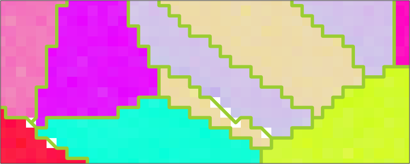

The yellow-green staircase is the measured boundary in the area used throughout the page. Its steps follow the square measurement grid rather than the physical boundary direction.

Step 1: remove the grid staircase

For an ideal straight boundary, the staircase is never farther than d/sqrt(2) from the line it approximates. The worst case is a boundary at 45 degree, whose corners lie exactly that far from the diagonal. simplifyBoundary therefore uses this as its default tolerance. It drops a vertex when removing it moves the boundary by less than the tolerance.

This argument separates the ideal grid staircase from features at larger scales. It cannot distinguish a real feature at the grid scale from a sampling artefact.

grainsSimple = simplifyBoundary(grains,d/sqrt(2));

plot(grains.boundary,'linewidth',5,'linecolor','YellowGreen','micronbar','off')
hold on
plot(grainsSimple.boundary,'linewidth',2,'linecolor','Fuchsia')
hold off
axis([313 353 140 156])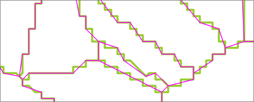

The magenta boundary has lost the staircase and is much shorter. It also has far fewer vertices because essentially only the corners have survived.

fprintf(['simplifying at a tolerance of %.2f %s takes the boundary' ...
  ' from %d segments to %d\n'],d/sqrt(2),grains.scanUnit, ...
  length(grains.boundary),length(grainsSimple.boundary))

simplifying at a tolerance of 0.71 um takes the boundary from 21269 segments to 5229

Step 2: restore evenly spaced samples

Smoothing the simplified result directly would be a mistake. A curved chain is now represented by a few long chords, and a Laplacian cuts the corners from the polygon they form. A circle with a radius of 15 pixels loses 14% of its area over 25 iterations that way, compared with 0.4% when this resampling step is included.

refineBoundary resamples each chain at equal arc length. It changes only the sampling, not the polygonal shape. The smoothing stage then receives evenly spaced degrees of freedom that are no longer tied to the measurement grid.

grainsRefined = refineBoundary(grainsSimple,d);

fprintf('resampling at %.2f %s puts them back: %d segments to %d\n', ...
  d,grains.scanUnit,length(grainsSimple.boundary), ...
  length(grainsRefined.boundary))

resampling at 1.00 um puts them back: 5229 segments to 18452

Step 3: smooth the resampled boundary

Only now does the filter move the boundary. A junction is a vertex where the number of meeting segments is not two. Junctions remain fixed by default.

grainsSmooth = smoothBoundary(grainsRefined,5,'noSimplify','noRefine');

plot(grains.boundary,'linewidth',5,'linecolor','YellowGreen','micronbar','off')
hold on
plot(grainsSmooth.boundary,'linewidth',2,'linecolor','Fuchsia')
hold off
axis([313 353 140 156])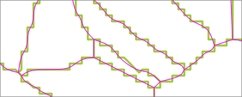

The magenta trace now follows the larger turns of the measured boundary without reproducing its pixel-scale steps.

These three stages are exactly what smoothBoundary(grains,5) performs. Both tolerances come from the median segment length measured before the first stage. After simplification, that median describes the straightened runs rather than the pixel spacing. The tolerances may also be set explicitly.

grainsCoarse = smoothBoundary(grains,5,'simplify',d/sqrt(2),'refine',2*d);

fprintf('resampling at %.2f %s instead leaves %d segments\n', ...
  2*d,grains.scanUnit,length(grainsCoarse.boundary))

resampling at 2.00 um instead leaves 9396 segments

What preprocessing changes

Simplification and resampling change the number of boundary segments. A resampled segment no longer lies between one specific pair of EBSD measurements, so its row of gB.ebsdId no longer identifies the pixels on its two sides. Use 'noSimplify' and 'noRefine' when an analysis needs that per-segment association.

Smoothing also changes lengths, areas, directions, and curvatures. It is a measurement choice, not merely a plotting choice. Record the filter and its settings when comparing maps or reporting shape statistics.

Choose the filter

A boundaryFilter controls the third stage. laplaceFilter and taubinFilter apply a local averaging step a fixed number of times. Their effect therefore depends on how densely the boundary is sampled. curvatureFilter and huberFilter instead specify a smoothing length in map units, which does not change when the same sample is measured on a finer grid. That length makes the setting comparable between scans only when their spatial units and preprocessing are also comparable.

Do not expect to distinguish sensible settings by eye on this map. All four results lie within a line width of one another, but their sub-pixel differences appear in boundary statistics. The following examples therefore compare grain areas.

The reference has passed through simplification and resampling but not smoothing. In other words, zero below means zero filter iterations, not the original pixel boundary. Grains with reference areas no greater than 10*d^2 are excluded so that a few-pixel grain does not dominate the percentages.

ref = smoothBoundary(grains,0);
A0 = ref.area;
big = A0 > 10*d^2;
A0 = A0(big);

fprintf('area comparison uses %d of %d grains\n',nnz(big),length(ref))

area comparison uses 443 of 523 grains

The Laplace filter

laplaceFilter is the default. It replaces each movable vertex by a weighted local mean, iter times. It is fast and useful for plots, directions, and lengths, but repeated averaging pulls a convex grain inward. Nothing bounds that shrinkage.

aL5 = smoothBoundary(grains,5).area;
aL5 = aL5(big);
aL25 = smoothBoundary(grains,25).area;
aL25 = aL25(big);

fprintf('grain area, laplaceFilter\n')
fprintf(['   5 iterations %+6.2f%% on average,' ...
  ' %+6.1f%% for the worst grain\n'], ...
  100*mean((aL5-A0)./A0),100*min((aL5-A0)./A0))
fprintf(['  25 iterations %+6.2f%% on average,' ...
  ' %+6.1f%% for the worst grain\n'], ...
  100*mean((aL25-A0)./A0),100*min((aL25-A0)./A0))

grain area, laplaceFilter
   5 iterations  -0.67% on average,  -18.1% for the worst grain
  25 iterations  -2.43% on average,  -59.0% for the worst grain

The Taubin filter

taubinFilter follows every smoothing pass with a slightly larger unshrinking pass. This approximately gives the area back instead of letting the mean area drift downwards. Areas still change, so the method is shrinkage resistant rather than exactly area preserving.

aT5 = smoothBoundary(grains,taubinFilter(5)).area;
aT5 = aT5(big);
aT25 = smoothBoundary(grains,taubinFilter(25)).area;
aT25 = aT25(big);

fprintf('grain area, taubinFilter\n')
fprintf(['   5 iterations %+6.2f%% on average,' ...
  ' %+6.1f%% for the worst grain\n'], ...
  100*mean((aT5-A0)./A0),100*min((aT5-A0)./A0))
fprintf(['  25 iterations %+6.2f%% on average,' ...
  ' %+6.1f%% for the worst grain\n'], ...
  100*mean((aT25-A0)./A0),100*min((aT25-A0)./A0))

grain area, taubinFilter
   5 iterations  -0.04% on average,   -2.2% for the worst grain
  25 iterations  -0.09% on average,   -6.9% for the worst grain

On this small grain, the Laplace result in magenta cuts inside the measured staircase. The Taubin result in blue follows it more closely.

A = grains.area;
[~,id] = min(abs(A-30));
c = grains(id).centroid;

plot(grains.boundary,'linewidth',4,'linecolor','LightGray','micronbar','off')
hold on
plot(smoothBoundary(grains,25).boundary, ...
  'linewidth',2.5,'linecolor','Fuchsia')
plot(smoothBoundary(grains,taubinFilter(25)).boundary, ...
  'linewidth',2.5,'linecolor','DodgerBlue')
hold off
axis([c.x-12 c.x+12 c.y-12 c.y+12])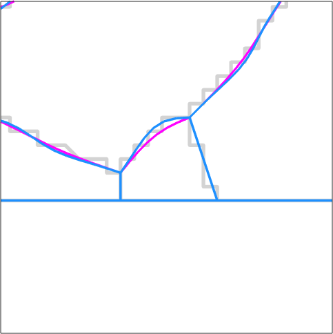

The curvature filter

curvatureFilter has no iteration count. smoothingLength is the wavelength damped to half amplitude, in the units of the map. Detail finer than that length is suppressed more strongly, and coarser detail survives. This gives the parameter a physical meaning that an iteration count does not have.

F = curvatureFilter;
F.smoothingLength = 8*d;

aC = smoothBoundary(grains,F).area;
aC = aC(big);

fprintf('grain area, curvatureFilter at a smoothing length of %.1f %s\n', ...
  8*d,grains.scanUnit)
fprintf('  %+6.2f%% on average, %+6.1f%% for the worst grain\n', ...
  100*mean((aC-A0)./A0),100*min((aC-A0)./A0))

grain area, curvatureFilter at a smoothing length of 8.0 um
   -0.26% on average,  -19.8% for the worst grain

The Huber filter

huberFilter uses the same smoothing length but protects sharp corners. Gentle undulations are smoothed like curvatureFilter, while a genuinely faceted boundary keeps its facets. This protection can also preserve corners left by the pixel grid on a boundary that is really straight or smooth. Reach for this filter when the material is faceted, not by default.

threshold is the turning angle at one vertex of the result, not the total angle of a corner. Smoothing first spreads a corner over roughly smoothingLength/h vertices, where h is their spacing. The Huber step then sharpens it again. For a rasterized hexagon with smoothingLength = 8*h, measured 60 degree corners return as follows.

A threshold of 15 degree is appropriate for the halfQuadraticFilter on orientations, but it would never activate corner protection here. The default boundary threshold is 5 degree.

G = huberFilter;
G.smoothingLength = 8*d;

aH = smoothBoundary(grains,G).area;
aH = aH(big);

fprintf('grain area, huberFilter at the same smoothing length\n')
fprintf('  %+6.2f%% on average, %+6.1f%% for the worst grain\n', ...
  100*mean((aH-A0)./A0),100*min((aH-A0)./A0))

grain area, huberFilter at the same smoothing length
   -0.16% on average,   -7.5% for the worst grain

A synthetic Voronoi map provides a case whose boundaries are exactly straight. On that map, huberFilter doubles the scatter of the boundary directions compared with curvatureFilter because it protects raster corners as if they were facets. This is the cost of preserving real corners.

Moving junctions

By default, all junctions remain fixed. The grains that touch and the junction positions therefore stay unchanged. Despite its name, 'moveTriplePoints' releases every non-outer junction, not only triple points. The outer map boundary remains fixed unless 'moveOuterBoundary' is also passed.

iter = [1 5 10 25];
color = copper(length(iter)+1);
dir = cell(size(iter));

plot(grains.boundary,'linewidth',1,'linecolor','LightGray','micronbar','off')
for i = 1:length(iter)
  gs = smoothBoundary(grains,iter(i),'moveTriplePoints');
  hold on
  plot(gs.boundary('i','i'),'linewidth',2,'linecolor',color(i,:))
  dir{i} = gs.boundary('i','i').direction;
end
hold off
axis([313 353 140 156])
mtexTitle('1, 5, 10, and 25 iterations: dark to light')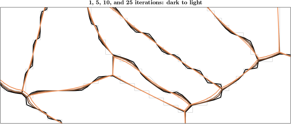

As the colour lightens, the released junctions move and the grid staircase is suppressed a little further. A Laplacian provides no barrier against collapse, however, so this freedom can let a small grain shrink away.

The direction histograms show the same progression. Each bar is weighted by segment length, and each panel is labelled with its iteration count. The radial scales differ, so compare the angular shapes rather than the absolute bar heights.

figure
for i = 1:length(dir)
  subplot(2,2,i)
  histogram(dir{i},'weights',norm(dir{i}),180)
  mtexTitle(sprintf('%d iterations',iter(i)))
end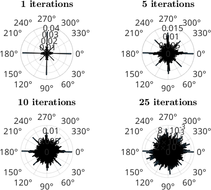

The maths behind the filters

The normalized boundary Laplacian L measures how far a vertex lies from the mean of its neighbours. The Laplace filter applies a low-pass step with gain \(1-\lambda k\). Its adjacency includes the vertex itself with the weight of its degree. A vertex with two neighbours therefore uses (2*V + Vl + Vr)/4. The documented default lambda = 0.5 consequently acts at a rate of 0.25. The 'gauss', 'exp', and 'umbrella' kernels reweight this adjacency by neighbour distance.

The Taubin filter follows that step with a negative step mu. The gain of a pair is \((1-\lambda k)(1-\mu k)\), which is approximately one at low frequencies when mu is chosen slightly larger in magnitude than lambda. High-frequency boundary steps are damped while broad shape is restored.

The curvature filter instead finds the vertices \(\mathbf{V}\) that minimize

\[\|\mathbf{V}-\mathbf{V}_0\|^2 + \alpha\|L\mathbf{V}\|^2.\]

The minimizer comes from one sparse linear system. Fixed junctions are eliminated from that system rather than penalized, so they stay exactly in place. On vertices sampled at spacing \(h\), the filter gain is \(1/(1+4\alpha\sin^4(\omega/2))\). The value of smoothingLength is the wavelength damped to half amplitude. Using the exact inverse rather than a small-angle approximation matters at short wavelengths: the approximation is already 20% wrong at four times the spacing. The implemented cutoff is within 0.05% of the requested value from three to 400 times the spacing.

The Huber filter replaces the squared curvature penalty with a Huber function. It is quadratic below threshold and linear above it. A least-squares penalty spreads a large turn over many vertices and rounds a corner. A linear, \(\ell^1\)-like penalty concentrates the turn into fewer vertices and preserves the corner. MTEX solves this problem by iteratively reweighted least squares until it converges. The iterMax property is a safety limit, not a smoothing control.

Further reading

Douglas and Peucker introduced the line-reduction algorithm used in the first stage: Algorithms for the Reduction of the Number of Points Required to Represent a Digitized Line or Its Caricature (1973).

Taubin developed the shrinkage-resistant signal-processing filter: A Signal Processing Approach to Fair Surface Design (1995).

The corner-preserving penalty comes from Huber's robust loss: Robust Estimation of a Location Parameter (1964).

For area-derived EBSD grain-size reporting, see ISO 13067:2020, Microbeam analysis - Electron backscatter diffraction - Measurement of average grain size. The standard concerns two-dimensional sectional measurements; it does not turn a smoothing choice into a three-dimensional measurement.

Related measurements

Boundary Curvature shows how geometric smoothing affects curvature. Shape Parameters develops the grain areas, perimeters, and shape descriptors that make filter choice a quantitative part of an analysis.

Next

Continue with Inferring Twin Boundaries, where a smoothed boundary network is classified by the misorientations across it.