Approximating Orientation Dependent Functions from Discrete Data

Approximating Orientation Dependent Functions from Discrete Data edit page

On this page we consider the problem of determining a smooth orientation dependent function \(f(\mathtt{ori})\) given a list of orientations \(\mathtt{ori}_n\) and a list of corresponding values \(v_n\). These values may be the volume of crystals with a specific orientation, as in the case of an ODF, or any other orientation dependent physical property.

Orientation dependent data may be stored in ASCII files with lines of Euler angles, representing the orientations, and values. Such data files can be imported by the command orientation.load, where we have to specify the position of the columns of the Euler angles as well as of the additional properties.

fname = fullfile(mtexDataPath, 'orientation', 'dubna.csv');
[ori, S] = orientation.load(fname,'columnNames',{'phi1','Phi','phi2','values'});

As a result the command returns a list of orientations ori and a struct S. The struct contains one field for each additional column in our data file. In our toy example it is the field S.values. Lets generate a discrete plot of the given orientations ori together with the values S.values.

plotSection(ori, S.values,'all','sigma');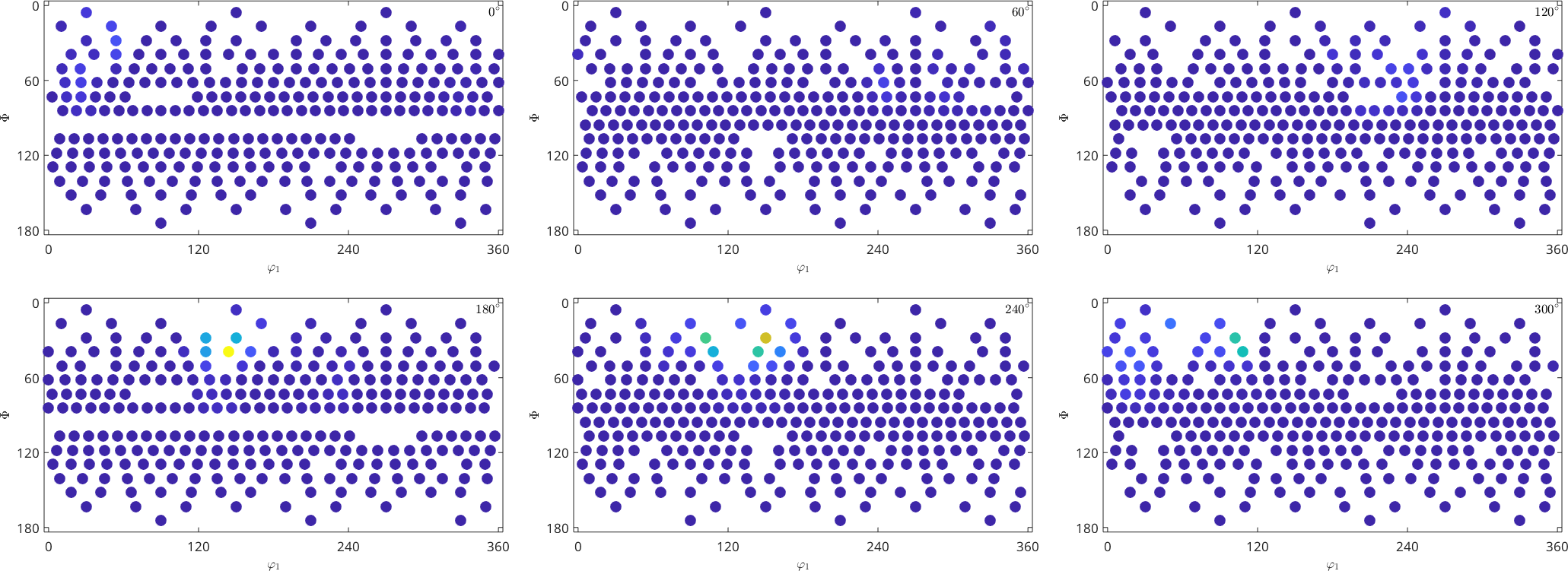

The process of finding a function which coincides with the given function values in the nodes reasonably well is called approximation. MTEX support different approximation schemes: approximation by harmonic expansion, approximation by radial functions and approximation by a Bingham distribution.

Approximation by Harmonic Expansion

An approximation by harmonic expansion is computed by the command SO3FunHarmonic.approximation

% SO3F = SO3Fun.interpolate(ori,S.values,'harmonic')
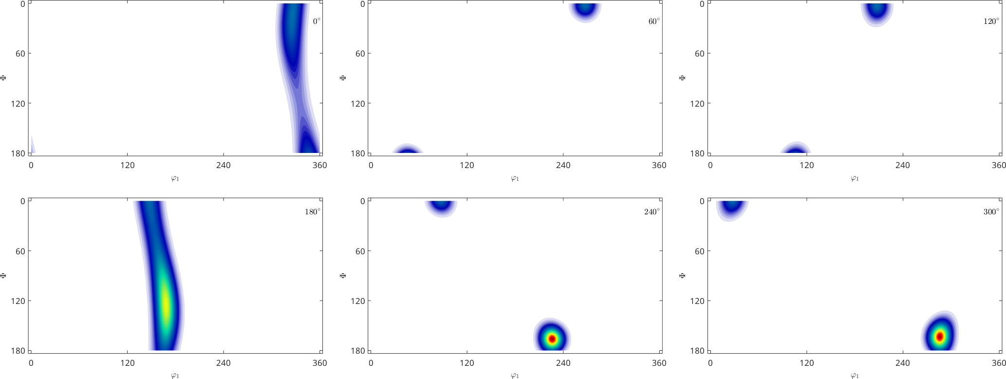
SO3F = SO3FunHarmonic.approximation(ori,S.values)
plot(SO3F,'sigma')

SO3F = SO3FunHarmonic (1 → xyz)
  bandwidth: 30
  weight: 0.99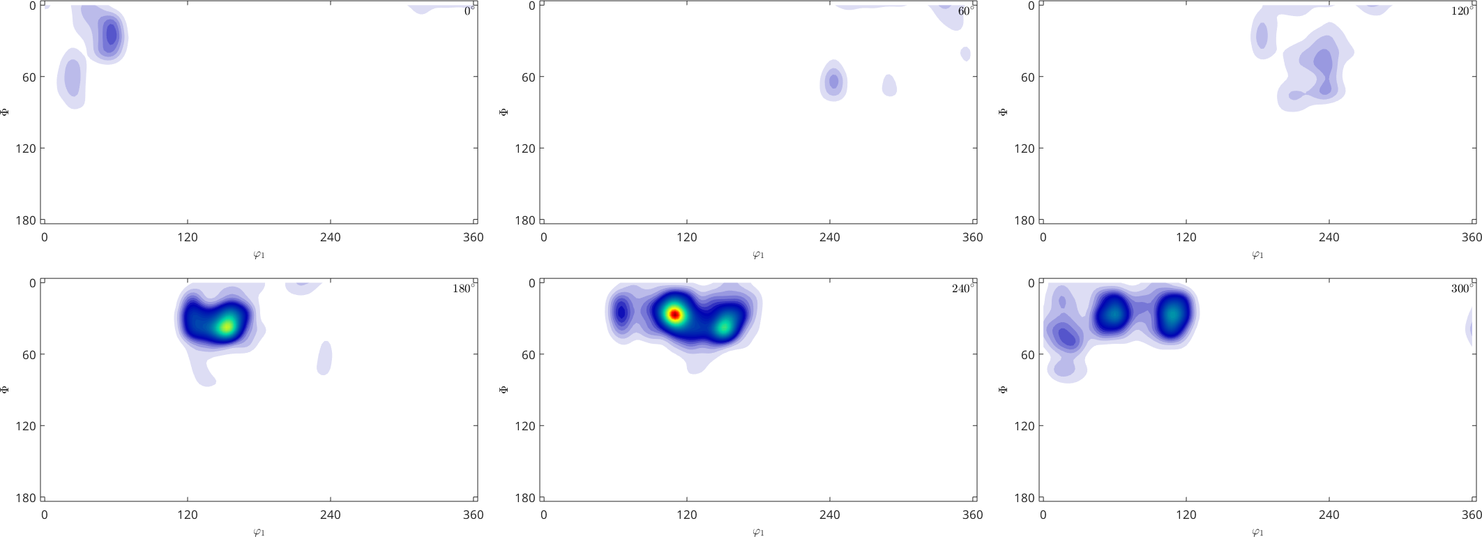

Note that SO3FunHarmonic.approximation does not aim at replicating the values exactly. In fact the relative error between given data and the function approximation is

norm(SO3F.eval(ori) - S.values) / norm(S.values)

ans =
    0.7743

The reason for this difference is that MTEX by default applies regularization. The default regularization parameter is \(\lambda = 0.0001\). We can switch off regularization by setting this value to \(0\).

SO3F = SO3FunHarmonic.approximation(ori,S.values,'regularization',0)

% the relative error
norm(SO3F.eval(ori) - S.values) / norm(S.values)

plot(SO3F,'sigma')

SO3F = SO3FunHarmonic (1 → xyz)
  bandwidth: 30
  weight: 0.67
 
ans =
   8.8649e-07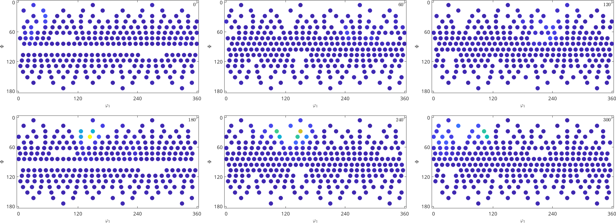

We observe that the relative error is much smaller, however the oscillatory behavior of the approximated function indicates overfitting. A more detailed discussion about choosing a good regularization parameter can be found in the section harmonic approximation theory.

An alternative way of regularization is to reduce the harmonic bandwidth

SO3F = SO3FunHarmonic.approximation(ori,S.values,'bandwidth',16)

% the relative error
norm(SO3F.eval(ori) - S.values) / norm(S.values)

plot(SO3F,'sigma')

SO3F = SO3FunHarmonic (1 → xyz)
  bandwidth: 16
  weight: 1
 
ans =
    0.7752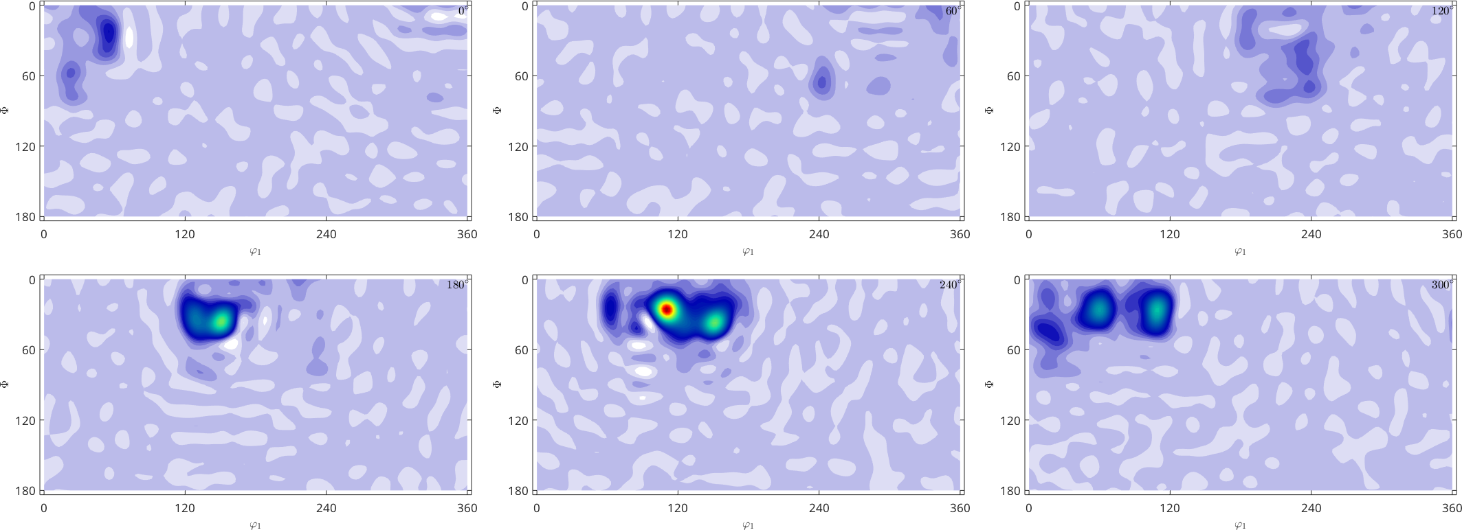

One big disadvantage of harmonic approximation is that the resulting function is not guarantied to be non negative, even if all given function values have been non negative.

min(SO3F)

ans =
   -0.5800

This possibility to guaranty non negativity is the central advantage of kernel based approximation.

Approximation by Radial Functions

The command for approximating orientation dependent data by a superposition of radial functions is SO3FunRBF.approximation.

% SO3F = SO3Fun.interpolate(ori,val,'odf');
SO3F = SO3FunRBF.approximation(ori,S.values,'odf');

% the relative error
norm(SO3F.eval(ori) - S.values) / norm(S.values)

plot(SO3F,'sigma')

Warning: Maximum number of iterations reached, result may not have converged to
the optimum yet. 
ans =
    0.0125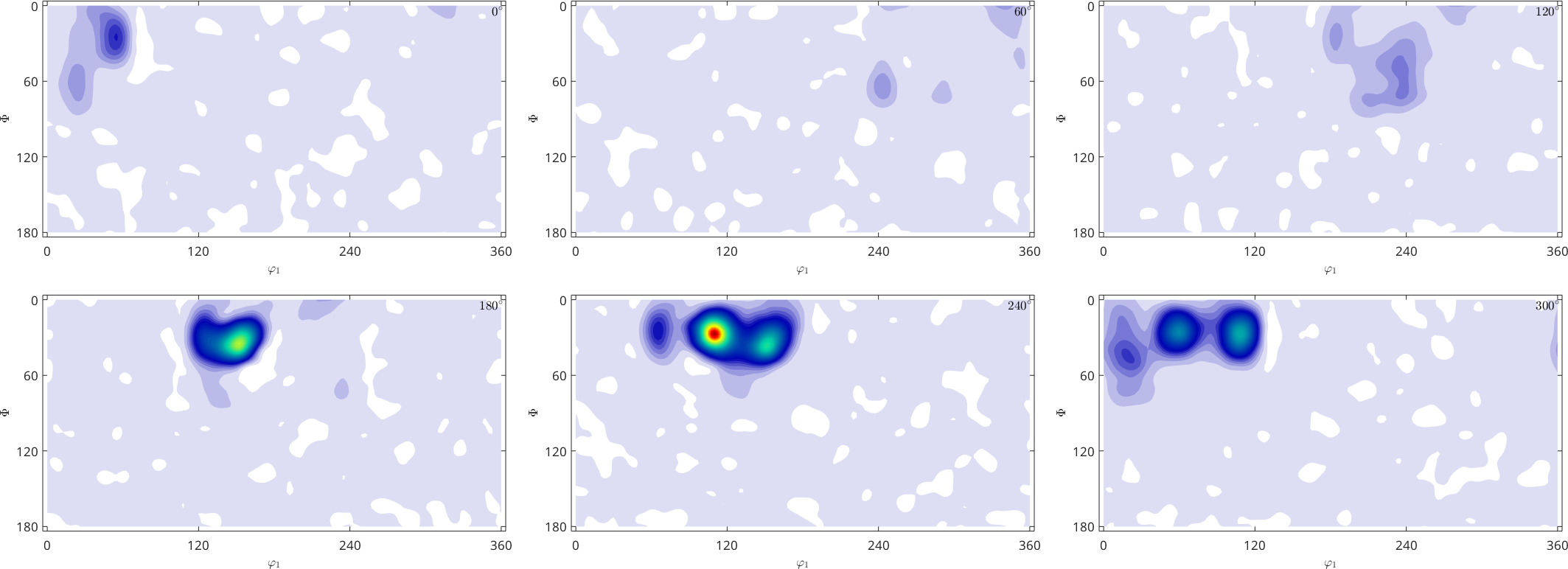

The option 'ODF' ensures that the resulting function is nonnegative and is normalized to \(1\)

min(SO3F)

mean(SO3F)

ans =
     0
ans =
    1.0000

The key parameter when approximation by radial functions is the halfwidth of the kernel function. This can be set by the option 'halfwidth'. A large halfwidth results in a very smooth approximating function whereas a very small halfwidth may result in overfitting

SO3F = SO3FunRBF.approximation(ori,S.values,'halfwidth',2.5*degree,'odf');

plot(SO3F,'sigma')

Warning: Maximum number of iterations reached, result may not have converged to
the optimum yet.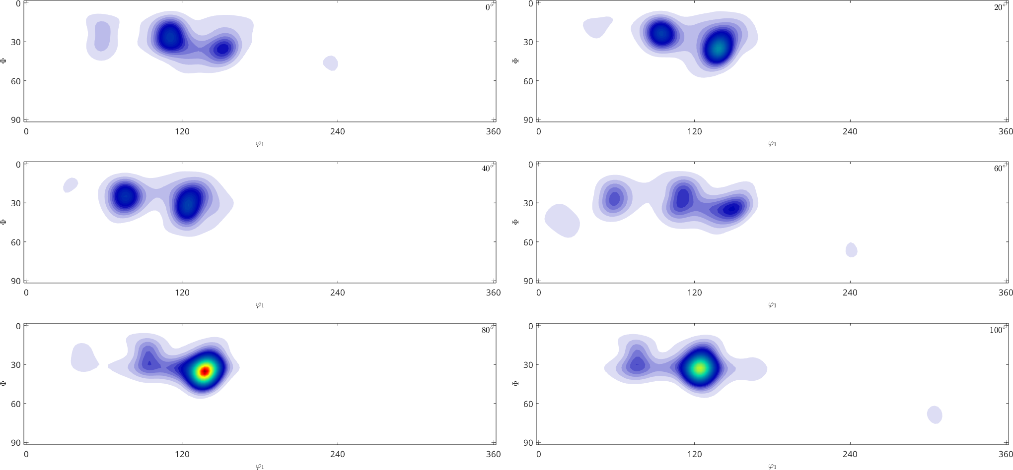

A more detailed discussion about the correct choice of the halfwidth and other options can be found in the section theory of RBF approximation.

If we omit the option 'odf' the resulting function may have negative values similar to the harmonic setting

SO3F = SO3FunRBF.approximation(ori,S.values);

% the relative error
norm(SO3F.eval(ori) - S.values) / norm(S.values)

plot(SO3F,'sigma')

ans =
    0.0313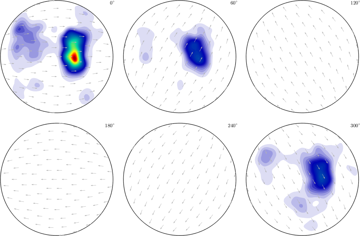

Approximating using the Bingham distribution

Approximation with the Bingham distribution currently works only with no symmetry. TODO!

cs = crystalSymmetry("1");
ori = equispacedSO3Grid(cs)

odf = fibreODF(fibre.rand(ori.CS))

figure(1)
plot(odf)

ori = SO3Grid (1 → xyz)
  grid: 119088 orientations, resolution: 5°
 
odf = SO3FunCBF (1 → xyz)
 
  kernel: de la Vallee Poussin, halfwidth 10°
  fibre : (71-1) || -9,4,1
  weight: 1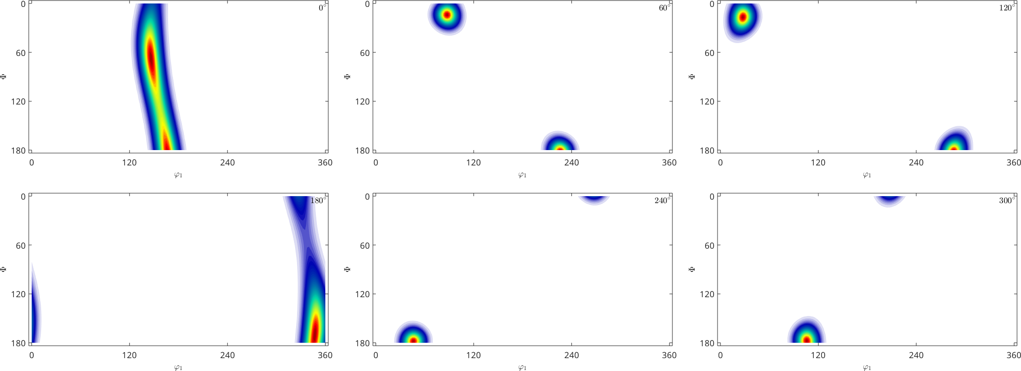

SO3F = calcBinghamODF(ori,'weights',odf.eval(ori))

figure(2)
plot(SO3F)

SO3F = SO3FunBingham (1 → xyz)
 
  kappa: 0 0.066 92 93
  weight: 1