Unlike most other texture analysis software MTEX does not have any graphical user interface. Instead the user is supposed to write scripts. Those scripts usually have the following structure
- import data
- inspect the data
- correct the data
- analyze the data
- plot and export the results of the analysis
During all these steps the data are stored as variables of different type. There are many different types of variables (called classes) for different objects, like vectors, rotations, EBSD data, grains or ODFs. The sidebar on the left lets you browse through all different MTEX class and the corresponding functions.
Variables are generated automatically when data are imported. E.g., the commands
fileName = [mtexEBSDPath filesep 'Forsterite.ctf'];
ebsd = EBSD.load(fileName,'EulerCorrection',rotation.byAxisAngle(xvector,180*degree))
ebsd = EBSD (y↑→x)
Phase Orientations Mineral Color Symmetry Crystal reference frame
0 58485 (24%) notIndexed
1 152345 (62%) Forsterite LightSkyBlue mmm
2 26058 (11%) Enstatite DarkSeaGreen mmm
3 9064 (3.7%) Diopside Goldenrod 12/m1 X||a*, Y||b*, Z||c
Properties: bands, bc, bs, error, mad
Scan unit : um
X x Y x Z : [0, 36550] x [0, 16750] x [0, 0]
Normal vector: (0,0,1)imports data from the file fileName.ctf and stores them in the variable ebsd of type EBSD.
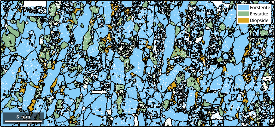
Next one can pass the variable ebsd to different MTEX function. For generating a phase plot is as simple as
plot(ebsd)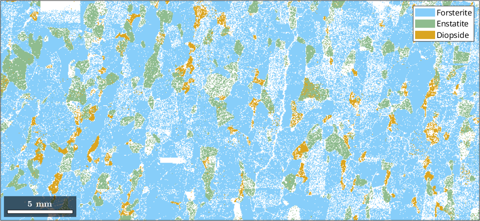
The grain structure is reconstructed by the command
grains = calcGrains(ebsd,'minPixel',5)grains = grain2d (y↑→x)
Phase Grains Pixels Mineral Symmetry Color
0 1410 37503 notIndexed
1 711 147812 Forsterite mmm LightSkyBlue
2 303 23896 Enstatite mmm DarkSeaGreen
3 175 6826 Diopside 12/m1 Goldenrod
boundary segments: 69817 (3.3e+06 µm)
inner boundary segments: 129 (5601 µm)
triple points: 3151
Properties: meanRotation, GOSwhich returns a new variable of type grain2d, here called grains. This variable contains the entire grain structure. Finally, we my visualize this structure by
hold on
plot(grains.boundary,'linewidth',2)
hold off