EBSD Tutorial

This tutorial follows one EBSD map from import to phase and orientation maps, reconstructed grains, pole figures, and inverse pole figures. It is a first route through MTEX rather than a guide to every choice.

Read General Concepts first if MTEX objects and selections are new to you. For your own data, read Reference Frame before trusting any orientation-dependent result.

from mtex import *

Data import

MTEX reads text formats such as .ang and .ctf and open binary formats such as .osc and .h5. The import chapter lists the supported formats and the information that may be missing from them.

The interactive import wizard, importWizard(), previews the file and writes a reproducible import script:

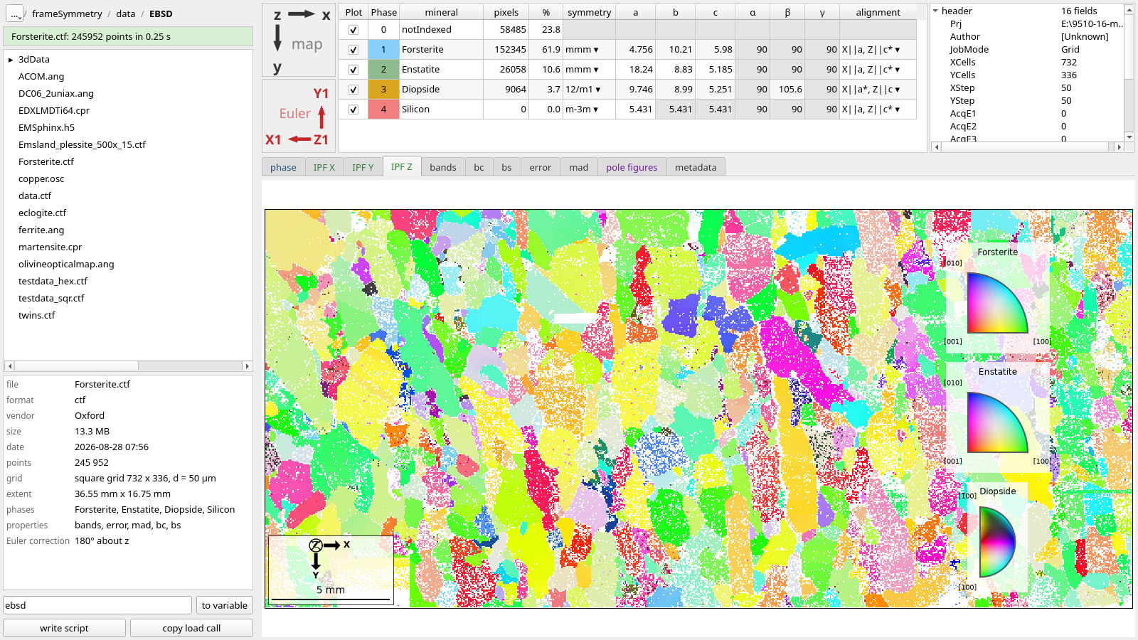
Notice the separate phase table, file header, map preview, and map and Euler reference-frame selectors. Check all four before asking the wizard to generate the script.

The generated script ultimately calls EBSD.load. Here the file and its Euler correction are known because both are packaged with MTEX:

# load example data packaged with MTEX
fileName = mtexdatafile('forsterite')
EulerCorrection = rotation.byAxisAngle(xvector, 180 * degree)
ebsd = EBSD.load(fileName, eulerCorrection=EulerCorrection)

ebsd

EBSD (y↓→x)
  size: 336 × 732 grid
  Phase  Orientations  Mineral     Color         Symmetry  Crystal reference frame
  0      58485 (24%)   notIndexed
  1      152345 (62%)  Forsterite  LightSkyBlue  mmm       Forsterite
  2      26058 (11%)   Enstatite   DarkSeaGreen  mmm       Enstatite
  3      9064 (3.7%)   Diopside    Goldenrod     12/m1     Diopside
  properties    : bands, bc, bs, error, mad
  scan unit     : um
  X × Y         : [0 → 3.655e+04] × [0 → 1.675e+04]
  square lattice: spacing 50

The correction above is specific to this file; do not copy it blindly to another data set. The displayed EBSD summary is the import audit: it lists the phases, counts, crystal symmetries, scan extent, and stored columns.

An EBSD object is a vectorized list with one entry per measurement, not an image. Its properties in ebsd.prop are per-pixel values that remain aligned when the map is subset. Its options in ebsd.opt contain scan-level information such as headers.

Phase map

With no colour data supplied, plot colours the measurements by phase. The reference-frame indicator is switched on for the first check.

plot(ebsd, refFrame='on')

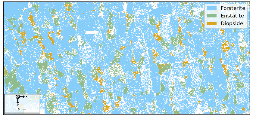
Forsterite dominates, while enstatite and diopside form separate regions. The white measurements have the phase notIndexed because their diffraction patterns could not be indexed; they are not missing pixels.

The corner indicator shows how the specimen frame is laid out on screen. A reference frame is the coordinate system in which the data is expressed, and it is distinct from the crystal symmetry of any phase.

Orientation map

Each phase has its own crystal symmetry, so select one phase before asking for an orientation array. The selection itself displays how many measurements it contains:

ebsd['Forsterite']

EBSD (y↓→x)
  size: 152345
  Phase  Orientations   Mineral     Color         Symmetry  Crystal reference frame
  1      152345 (100%)  Forsterite  LightSkyBlue  mmm       Forsterite
  properties    : bands, bc, bs, error, mad
  scan unit     : um
  X × Y         : [0 → 3.655e+04] × [0 → 1.675e+04]
  square lattice: spacing 50

Its orientations form another vectorized object. The display confirms its size and its crystal and specimen frames:

ebsd['Forsterite'].orientations

orientation (Forsterite → y↓→x)
  size: 152345
  Bunge Euler angles in degree
  phi1   Phi  phi2
  95.3  42.3   294
  95.6  42.3   293
  95.4  42.4   294
  95.6  42.2   293
  95.4  42.3   294
     ⋮     ⋮     ⋮
   180    53   239
   180  52.6   239
   180  52.8   243
   180  52.7   242
   180  52.7   242

Passing those orientations as the colour data produces an inverse pole figure map.

plot(ebsd['Forsterite'], ebsd['Forsterite'].orientations, micronbar='off')

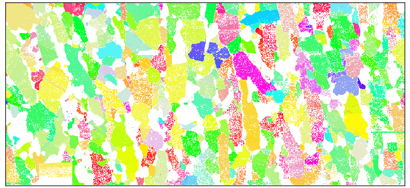
Similar colours suggest similar orientations, but a colour patch is not a grain. The default IPF-Z key is a projection, so it can hide orientation differences, and a real grain may contain a smooth orientation gradient. See IPF Maps to draw and choose the colour key explicitly.

Grain reconstruction

This packaged example goes directly from import to segmentation. For a real map, inspect its quality properties and use Select to isolate suspect measurements first. Denoising and Filling Missing Data change the map and need a specimen-specific justification.

calcGrains segments the measurement list into regions. A grain is a phase-homogeneous, spatially connected region of EBSD pixels produced by segmentation. A phase change is always a grain boundary, while same-phase neighbours are separated here when their misorientation exceeds the chosen angle. A connected notIndexed area can itself form a grain; it is not a gap in the scan.

The 10 degree angle is an example parameter, not a universal definition. The option minPixel removes indexed grains smaller than five pixels and marks their pixels notIndexed.

# reconstruct grains with a 10 degree misorientation angle
grains = calcGrains(ebsd, angle=10 * degree, minPixel=5)
grains

grain2d (y↓→x)
  size: 885
  Phase  Grains               Mineral     Color         Symmetry  Crystal reference frame
  0      20 (1381 pixels)     notIndexed
  1      489 (151487 pixels)  Forsterite  LightSkyBlue  mmm       Forsterite
  2      209 (25656 pixels)   Enstatite   DarkSeaGreen  mmm       Enstatite
  3      167 (7419 pixels)    Diopside    Goldenrod     12/m1     Diopside
  boundary segments: 36193, inner: 190, triple points: 1525

# smooth only the boundary geometry
grains = smoothBoundary(grains, 5)

The returned grain2d object is a vectorized list of grains. Its display reports the count by phase and the available grain properties. smoothBoundary removes the pixel staircase from the outlines; it does not change which measurements belong together. See Grain Reconstruction for choosing and testing segmentation criteria.

Overlaying the boundaries provides the first visual check:

# overlay the grain boundaries on the orientation map
hold(True)
plot(grains.boundary, lineWidth=2)
hold(False)

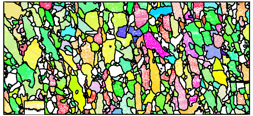
Most boundaries follow clear changes in orientation colour. Where they do not, inspect the colour key and the underlying misorientations rather than tuning the angle to the picture alone.

Crystal orientation glyphs

A crystal shape can be used as an orientation glyph. The predefined olivine polyhedron is rotated by each grain’s mean orientation and placed at its centroid.

# define an idealized olivine crystal shape
cS = crystalShape.olivine(ebsd['Forsterite'].CS)

# retain Forsterite grains with more than 100 measurements
grains = grains['Forsterite', grains.numPixel > 100]
grains

grain2d (y↓→x)
  size: 262
  Phase  Grains               Mineral     Color         Symmetry  Crystal reference frame
  1      262 (142943 pixels)  Forsterite  LightSkyBlue  mmm       Forsterite
  boundary segments: 24855, inner: 163, triple points: 1333

# overlay the oriented crystal glyphs
hold(True)
plot(grains, 0.7 * cS, colored=True)
hold(False)

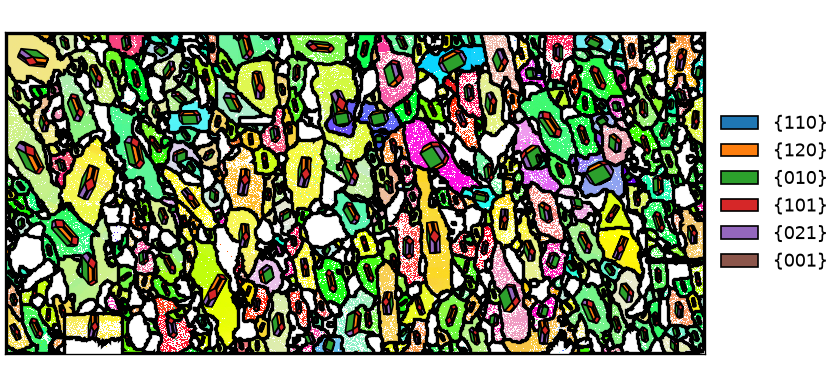
The grain summary above gives the number retained by the selection. The repeated face orientations reveal the preferred orientation, or texture, of this population.

These glyphs do not measure three-dimensional crystal habit or grain morphology; the shape is idealized and its linear scale follows the square root of grain area. See Crystal Shapes for constructing other glyphs.

Pole figures

A pole figure asks where a chosen crystal direction points in the specimen for every measured orientation. The command is plotPF. Here the three crystallographic axes are plotted as filled density contours.

# select three crystal directions
h = Miller([1, 0, 0], [0, 1, 0], [0, 0, 1], ebsd['Forsterite'].CS)

# plot their specimen-direction distributions
plotPF(ebsd['Forsterite'].orientations, h, contourf=True)
mtexColorbar()

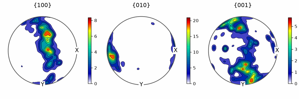
The (010) poles collect in a strong maximum near the rim. The (100) poles occupy a broad band, while the (001) poles form several concentrations. A random orientation population would be uniform apart from sampling variation, so these concentrations are evidence of texture.

Every measurement has equal weight in these plots. On a regular map this is area weighting, so large grains contribute more than small grains and the scanned area must represent the specimen.

Inverse pole figures

An inverse pole figure asks the complementary question: which crystal direction points along a chosen specimen direction? The command is plotIPF.

# select the specimen axes
r = vector3d.cat(vector3d.X, vector3d.Y, vector3d.Z)

# plot their crystal-direction distributions
plotIPF(ebsd['Forsterite'].orientations, r, contourf=True)
mtexColorbar()

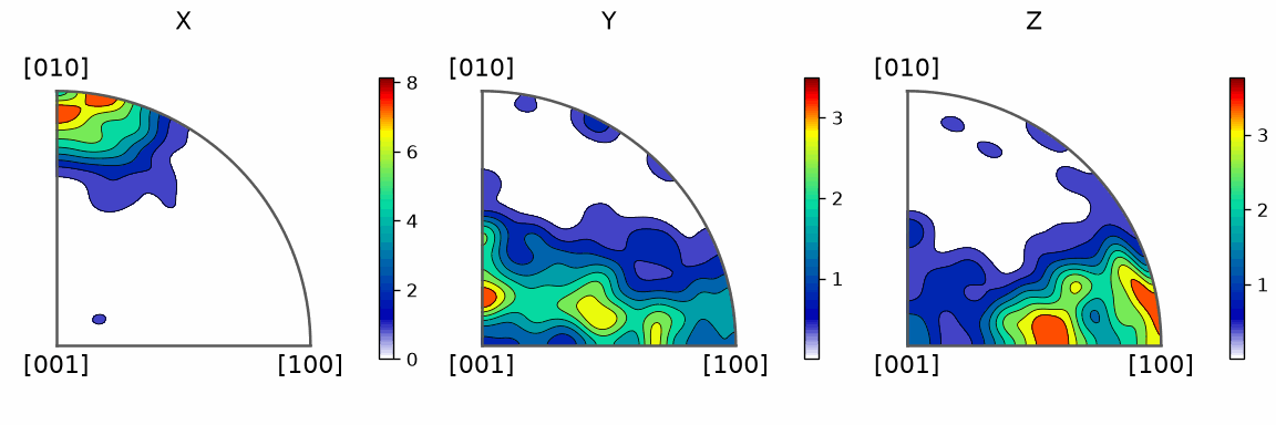
The strongest concentration for the specimen x axis lies toward the crystal [010] direction. This is the complementary view of the (010) pole-figure maximum. The y and z distributions are broader and lie mainly along the sector edge between [001] and [100].

Pole figures and inverse pole figures are projections of the same three-dimensional orientation data, and neither is a complete description. ODF Estimation explains how pixel weighting, grain weighting, and kernel choice affect a continuous orientation distribution.

Next

Continue with the grain tutorial to measure and select the reconstructed grains. Then use the grain boundary tutorial for the crystallographic relations between neighbouring grains.

For texture analysis, the ODF tutorial turns individual orientations into a function that can be evaluated, integrated, and compared.

Further reading

• A.J. Schwartz et al., editors, Electron Backscatter Diffraction in Materials Science, 2nd ed., Springer, 2009.
• T.B. Britton et al., Tutorial: Crystal orientations and EBSD - Or which way is up?. Mater. Charact. 117 (2016), 113-126.
• F. Bachmann et al., Grain detection from 2d and 3d EBSD data - Specification of the MTEX algorithm, Ultramicroscopy 111 (2011), 1720-1733.
• ISO 13067:2020 specifies EBSD procedures for measuring average grain size from two-dimensional sections.

Technical Details

calcGrains(ebsd, angle=10*degree, minPixel=5) gives 20, 489, 209 and 167 notIndexed, forsterite, enstatite and diopside grains and 36193 boundary segments where MATLAB has 9, 489, 208, 167 and 35402: the fragments the second segmentation leaves below minPixel are notIndexed grains here, and a small difference in the segmentation remains, as on the other forsterite pages. The 262 forsterite grains above 100 pixels agree, with 142943 pixels for MATLAB’s 142951.

@article{bachmann2010mtex,
  author  = {F. Bachmann and R. Hielscher and H. Schaeben},
  title   = {Texture Analysis with MTEX - Free and Open Source Software Toolbox},
  journal = {Solid State Phenomena},
  volume  = {160},
  pages   = {63-68},
  year    = {2010},
  doi     = {10.4028/www.scientific.net/SSP.160.63},
  url     = {https://doi.org/10.4028/www.scientific.net/SSP.160.63}
}