ODF Tutorial

An orientation distribution function (ODF) describes the texture of a specimen as a continuous density over all crystal orientations. It is the common result of two different experiments: orientation maps measure orientations individually, while diffraction measures pole figures.

Read General Concepts first if MTEX objects and selections are new to you. The EBSD tutorial introduces orientation maps, and the pole figure tutorial develops diffraction data.

MTEX reports ODF values in multiples of a random distribution, mrd. A random texture has value 1 everywhere. A value of 10 means ten times the random density near that orientation; it is not the volume fraction at one exact orientation.

This tutorial follows three routes to an ODF: estimate one from individual orientations, reconstruct one from pole figures, and define a model ODF.

from mtex import *

From individual orientations

The titanium map contains 8148 measurement points, but 48 could not be indexed and therefore have no orientation. Select the indexed titanium phase before estimating its density.

# load the titanium example without displaying the EBSD summary
ebsd = mtexdata('titanium', verbose=False)

# select the indexed orientations
titanium = ebsd['Titanium (Alpha)']
ori = titanium.orientations

# display the number of orientations used in the estimate
numOrientations = len(ori)
numOrientations

8100

# colour the map with one explicit inverse pole figure key
ipfKey = ipfColorKey(ori)
plot(titanium, ipfKey.orientation2color(ori))

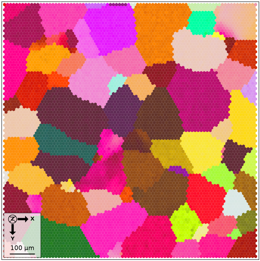
Reading the orientation map

The map contains broad regions of similar colour rather than 8100 independent colour speckles. Neighbouring EBSD pixels are spatially correlated because many sample the same crystal.

calcDensity uses kernel density estimation. It places a smooth kernel at every orientation and adds the kernels. The halfwidth controls how far each measurement is spread in orientation space; here it is set explicitly to 10 degrees.

halfwidth = 10 * degree
odfFromOrientations = calcDensity(ori, halfwidth=halfwidth)
odfFromOrientations

SO3FunHarmonic (Titanium (Alpha) → y↓→x)
  bandwidth: 25
  mean     : 1

Reading the ODF summary

The summary identifies an SO3FunHarmonic with bandwidth 25 and weight 1. Harmonic coefficients are its numerical representation, while the weight confirms that the ODF is normalized as one complete texture.

Compute the maximum instead of estimating it from a colour scale.

orientationODFMaximum, _ = max(odfFromOrientations, numLocal=1)
orientationODFMaximum

9.0003

# plot sigma sections for the hexagonal titanium phase
plot(odfFromOrientations, 'sigma')
mtexColorbar(title='orientation density (mrd)')

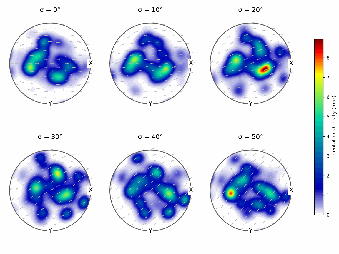
Reading the estimated ODF

The maximum is 9.0 mrd. In the sigma sections, the high-density region extends through neighbouring sections because the estimate is a continuous function rather than a list.

The 10 degree halfwidth is an analysis choice, not a property of titanium. A smaller value resolves finer structure and usually raises the maximum, while a larger value merges nearby features. Neither change is automatically more accurate.

The sampling weights matter as well. Pixel orientations weight mapped area, while grain mean orientations give every reconstructed grain one vote unless grain area is supplied as a weight. ODF Estimation develops halfwidth selection and weighting.

From pole figures

Diffraction does not measure individual orientations. For each lattice plane, it measures intensity over specimen directions. Load three orthorhombic pole figures and display their input summary.

plottingConvention.default('y↑→x')

# load the pole figure example
pf = mtexdata('ptx', verbose=False)
pf

PoleFigure (mmm → y↑→x)
  h = {104}, r = 72 × 17 points
  h = {110}, r = 72 × 17 points
  h = {202}, r = 72 × 17 points

# plot the measured intensities
plot(pf)
mtexColorbar(title='measured intensity')

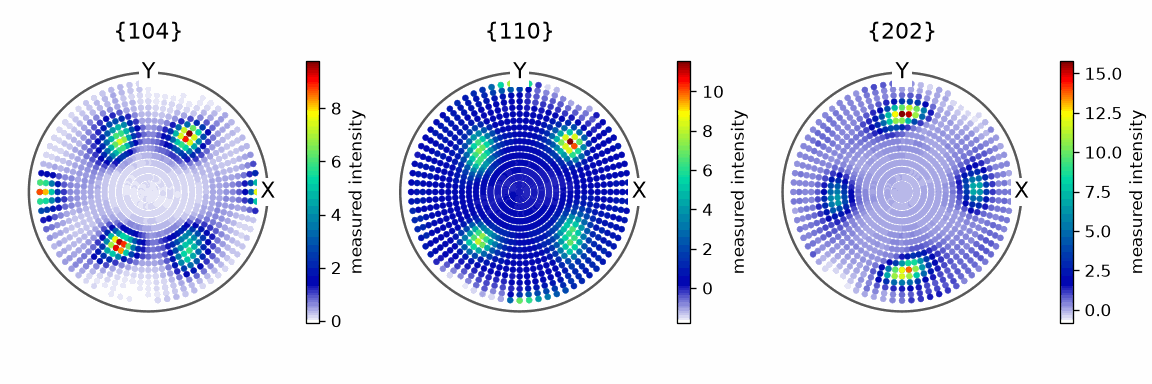
Reading the measured pole figures

The summary reports three grids of 72 by 17 specimen directions, for 3672 intensity values in total. The three plots have distinct spot patterns because each reflection places a different constraint on the unknown ODF.

calcODF finds an ODF whose recalculated pole figures fit those measurements. The silent flag hides the solver iteration table but leaves the returned ODF summary visible.

odfFromPoleFigures = calcODF(pf, verbose=False)
odfFromPoleFigures

SO3FunRBF (mmm → y↑→x)
  multimodal components
    kernel: de la Vallee Poussin, halfwidth 5°
    center: 29818 orientations
    weight: 1
    Bunge Euler angles in degree
    phi1  Phi  phi2    weight
      90  2.5   180  2.55e-05
      90  2.5   185  4.36e-05
      90  2.5   190  4.27e-05
      90  2.5   195  2.53e-05
      90  2.5   200  1.13e-05
       ⋮    ⋮     ⋮         ⋮
    35.2  107   305  8.88e-06
    40.4  107   310  1.66e-05
    45.7  107   314  3.33e-05
    50.9  107   319  3.58e-05
    56.1  107   324  1.84e-05

Reading the reconstructed ODF summary

This result is an SO3FunRBF, represented as a weighted sum of kernels on an orientation grid. It is the same scientific quantity as the harmonic ODF above despite the different representation.

poleFigureODFMaximum, _ = max(odfFromPoleFigures, numLocal=1)
poleFigureODFMaximum

17.2091

The maximum is about 17 mrd, so this reconstructed texture is sharper than the titanium estimate under their respective smoothing choices. Peak height alone should not be used to compare specimens unless the estimation and reconstruction settings are also comparable.

The first validation is to recalculate the measured reflections.

# plot pole figures recalculated from the ODF
plotPF(odfFromPoleFigures, pf.allH)
mtexColorbar(title='recalculated intensity')

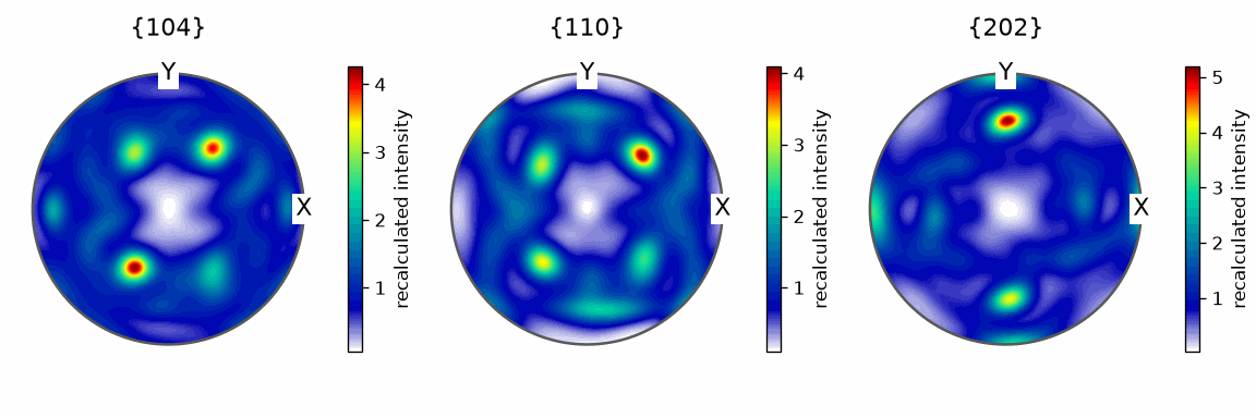
Reading the recalculated pole figures

The broad maxima occupy the same regions as in the measured plots above. The recalculated fields are smooth and do not reproduce every measured point-to-point fluctuation. A systematic shift or a missing maximum would instead indicate a problem with the input, reference frame, corrections, or reconstruction settings.

Agreement does not prove that the ODF is unique. Pole-figure inversion cannot recover every part of an ODF, even from noiseless measurements. The Ghost Effect explains the missing information, and Ghost Correction explains the additional assumption used by MTEX by default. Continue with ODF Reconstruction for solver choices and quantitative fit measures.

Model ODFs

An ODF need not come from measurements. A model ODF provides a known reference texture for interpretation, simulation, or comparison with an estimate.

The gamma fibre is a standard cubic rolling-texture component. Every orientation on its ideal curve places a crystal {111} plane normal parallel to the specimen normal direction. Define both symmetries explicitly so this model does not inherit anything from the orthorhombic diffraction example.

cs = crystalFrame('cubic')
ss = specimenFrame('orthorhombic')
gammaFibre = fibre.gamma(cs, ss)

# spread density by 10 degrees around the ideal gamma fibre
modelODF = fibreODF(gammaFibre, halfwidth=10 * degree)
modelODF

SO3FunCBF (m3̅m → y↑→x)
  fibre component
    kernel: de la Vallee Poussin, halfwidth 10°
    fibre : (111) || (0,0,1), weight 1
    weight: 1

modelODFMaximum, _ = max(modelODF, numLocal=1)
modelODFMaximum

11.4879

# use conventional Euler sections for this cubic rolling texture
plot(modelODF)
mtexColorbar(title='orientation density (mrd)')

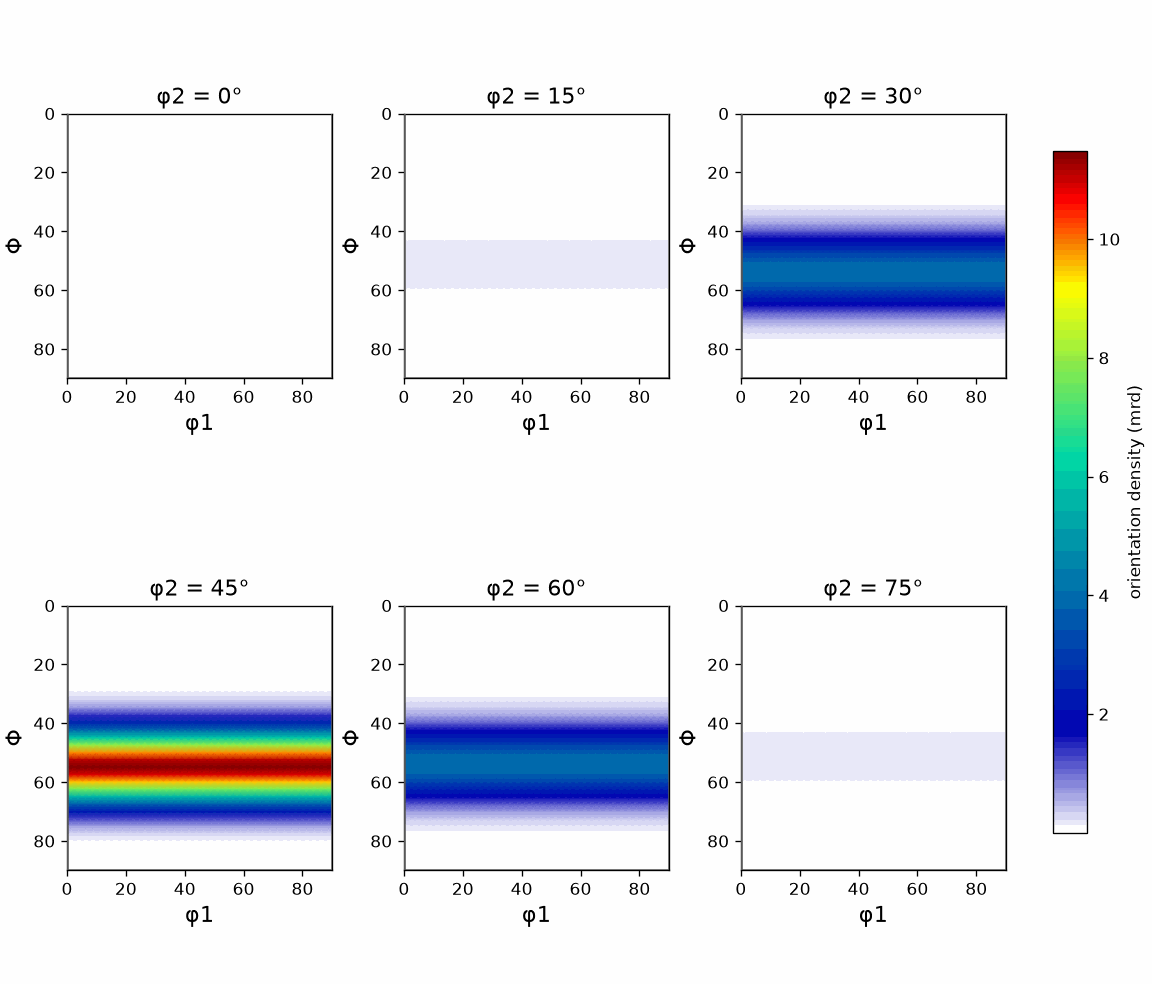
Reading the model ODF

The maximum is 11.5 mrd. The fibre shows up as a band running across the whole width of the \(\varphi_2 = 45^\circ\) section, not as an isolated peak. It is weaker in the neighbouring sections at 30 and 60 degrees and absent from the remaining three, so most of the density sits in a narrow range of \(\varphi_2\). The 10 degree kernel gives the band finite width, so this is a smooth model around an ideal fibre rather than density confined to a line.

Model ODFs combines uniform, unimodal, fibre, and Bingham components. Fibre ODFs develops the role of the halfwidth and the pole figures produced by a fibre.

One ODF interface

The three displays above report SO3FunHarmonic, SO3FunRBF, and SO3FunCBF. These class names describe storage and approximation strategies, not three definitions of texture. All implement the SO3Fun interface for evaluation, plotting, integration, extrema, rotation, arithmetic, and random sampling.

This common interface is how MTEX connects EBSD, pole figures, texture models, crystal-plasticity input, and anisotropic material properties. ODF Analysis develops plots, components, and scalar texture measures. Random Sampling turns any ODF back into discrete orientations, while Tensors uses an ODF to average direction-dependent crystal properties.

The maths behind the two data routes

For an orientation \(g\), the ODF is the normalized material-volume density

Its integral over orientation space is 1. With the uniform probability measure used by MTEX, the random ODF is therefore the constant function 1 and ODF values have units of mrd.

For measured orientations \(g_1,\ldots,g_N\) and a normalized kernel \(\psi\), kernel density estimation gives

The kernel halfwidth controls the smoothing described above. Crystal and specimen symmetries identify equivalent orientations in both the kernel and the domain.

A pole figure is instead a projection of the ODF. For a crystal direction \(h\) and specimen direction \(r\), its pole density integrates over the orientation fibre that maps \(h\) to \(r\):

Reconstructing an ODF from these projections is the inverse problem used by calcODF.

Further reading

• H.-J. Bunge, Texture Analysis in Materials Science: Mathematical Methods, Butterworths, English ed., 1982, develops classical ODF, pole-figure, and harmonic theory.
• H. Schaeben, A simple standard orientation density function: the hyperspherical de la Vallee Poussin kernel, Phys. Status Solidi B 200 (1997), 367-376.
• R. Hielscher and H. Schaeben, A novel pole figure inversion method: specification of the MTEX algorithm, J. Appl. Cryst. 41 (2008), 1024-1037.
• F. Bachmann, R. Hielscher and H. Schaeben, Texture Analysis with MTEX - Free and Open Source Software Toolbox, Solid State Phenomena 160 (2010), 63-68.
• ASTM E81-96(2024) covers X-ray acquisition of quantitative pole figures; it does not specify ODF inversion.

Technical Details

The titanium estimate agrees with MATLAB’s to the digit: 8100 orientations, bandwidth 25, maximum 9.0003 mrd, and the same sigma sections. The ptx reconstruction places its kernels on 29818 orientations where MATLAB’s equispaced grid has 29772. The solver stops after six iterations under MATLAB’s stopping rule, and its maximum, 17.21 mrd, is 3 percent below MATLAB’s 17.72 (MATLAB’s text quotes 17.8). The maximum is sensitive to the stopping point: five iterations give 12.8 mrd and seven give 23.8. The recalculated pole figures agree by eye. The model ODF, its display, its maximum 11.4879 (MATLAB 11.4878) and its sections agree.

@article{bachmann2010mtex,
  author  = {F. Bachmann and R. Hielscher and H. Schaeben},
  title   = {Texture Analysis with MTEX - Free and Open Source Software Toolbox},
  journal = {Solid State Phenomena},
  volume  = {160},
  pages   = {63-68},
  year    = {2010},
  doi     = {10.4028/www.scientific.net/SSP.160.63},
  url     = {https://doi.org/10.4028/www.scientific.net/SSP.160.63}
}