ODF Estimation from EBSD Data

An EBSD map records one orientation at every indexed measurement. That is a finite list of points, and a plot of that list shows where orientations occur but not how many. Answering how much of the specimen sits near an orientation needs a continuous density, and this page estimates one.

The page assumes phase selection from Select EBSD Data and the scatter plots of Plotting Individual Orientations. A reference frame is the coordinate system in which the data are expressed. Check it as described in Reference Frame before reading a specimen direction from any figure below.

A plotting convention states how that frame is laid out on screen. The convention below draws specimen Y upward and specimen X to the right. It changes the screen layout, not the measured orientations.

import numpy as np

from mtex import *

plottingConvention.default('y↑→x')
ebsd = mtexdata('copper')

# a density describes one phase, so select it first
copper = ebsd['copper']
ori = copper.orientations
ori

orientation (Copper → y↑→x)
  size: 16116
  Bunge Euler angles in degree
  phi1   Phi  phi2
  55.9  95.8   134
  56.4  94.3   135
   142  45.2    96
   2.7   104   205
  2.39   105   205
     ⋮     ⋮     ⋮
  7.14  86.3   189
   257  9.95   110
   180   120   136
   183  84.2   156
   183  84.2   156

ipfKey = ipfColorKey(copper)
plot(copper, ipfKey.orientation2color(ori))

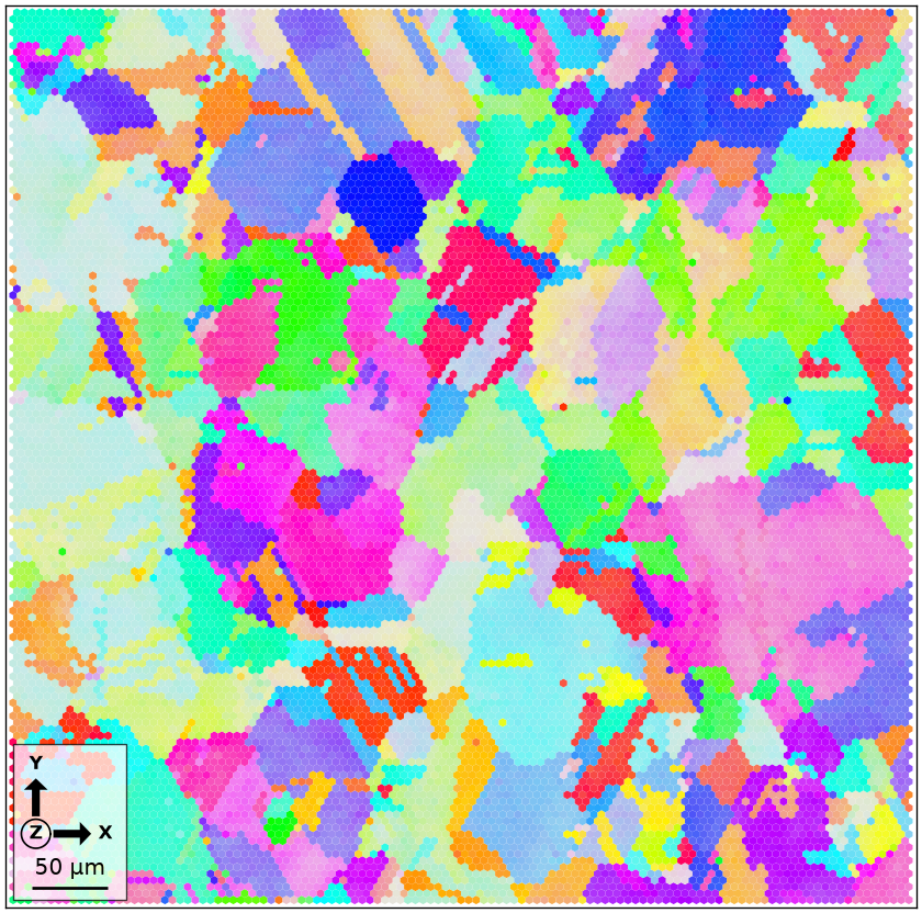
The list holds 16116 orientations. The IPF colours form broad patches, because neighbouring pixels of one grain repeat nearly the same orientation. A grain is a phase-homogeneous, spatially connected region of EBSD pixels produced by segmentation. This map contains a few hundred of them, so its 16116 orientations are far fewer than 16116 independent observations. That distinction decides everything below.

Start with the orientations themselves

A pole figure fixes a crystal direction and shows where it points in the specimen. Drawing one marker per measurement shows the data and nothing but the data.

h = cat(Miller(1, 0, 0, ori.CS), Miller(1, 1, 0, ori.CS), Miller(1, 1, 1, ori.CS))
plotPF(ori, h, antipodal=True, markerSize=2)

  I'm plotting 208 random orientations out of 16116 given orientations
  You can specify the number of points by the option "points".
  The option "all" ensures that all data are plotted

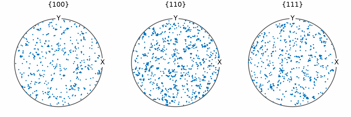
MTEX drew 208 of the 16116 orientations at random, since every one of them contributes several symmetrically equivalent poles and the full list would be an opaque blot. The option all=True overrides that, and points sets the sample size.

The markers cover the whole pole figure with faint clumping. Some directions are visibly more populated than others, but the plot gives no way to say how much more. Overlapping markers hide their own count, so two spots of equal appearance may differ by a factor of ten.

Sections through orientation space keep all three orientation coordinates instead of projecting one away.

plotSection(ori, 'sigma', sections=6, points=2000)

plot 2000 random orientations out of 16116 given orientations

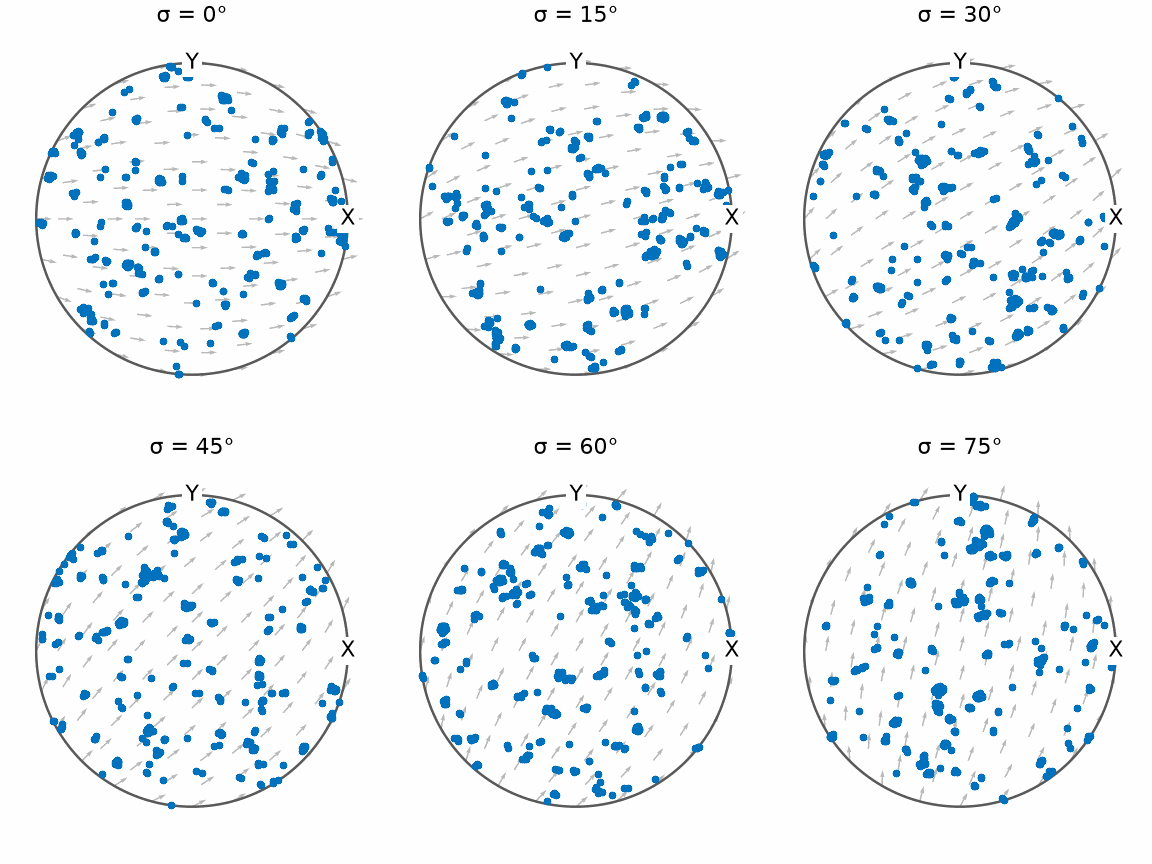
Now the structure of the sample is plain: the markers sit in tight knots of a dozen or more. Each knot is one grain measured many times, not a texture component observed many times. The knots can be seen but not counted, exactly as in the pole figure.

Contouring turns markers into values

Adding the option contourf replaces the markers by filled contours with a colour bar, so the plot finally carries numbers.

plotPF(ori, h, antipodal=True, contourf=True)
mtexColorbar(title='mrd')

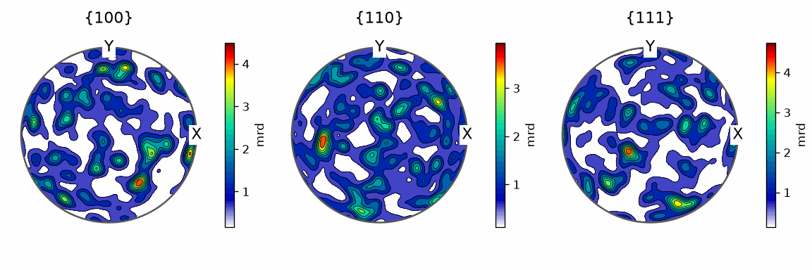
The unit is multiples of a random distribution (mrd). A uniform texture is 1 mrd everywhere, so 4 mrd means four times as many poles as a uniform specimen would put there. It is not a percentage of the specimen.

The colour bars top out between 3.7 and 4.7 mrd, spread over dozens of separate small spots rather than a few texture components.

Those values are not measured but estimated. MTEX places a small bell-shaped function, a kernel, on every plotted pole and adds the copies up. The width of that kernel is its halfwidth, the angular distance at which it falls to half its peak value. Left unspecified, the contoured pole figure uses 5 degrees. Ask for 15 degrees instead.

plotPF(ori, h, antipodal=True, contourf=True, halfwidth=15 * degree)
mtexColorbar(title='mrd')

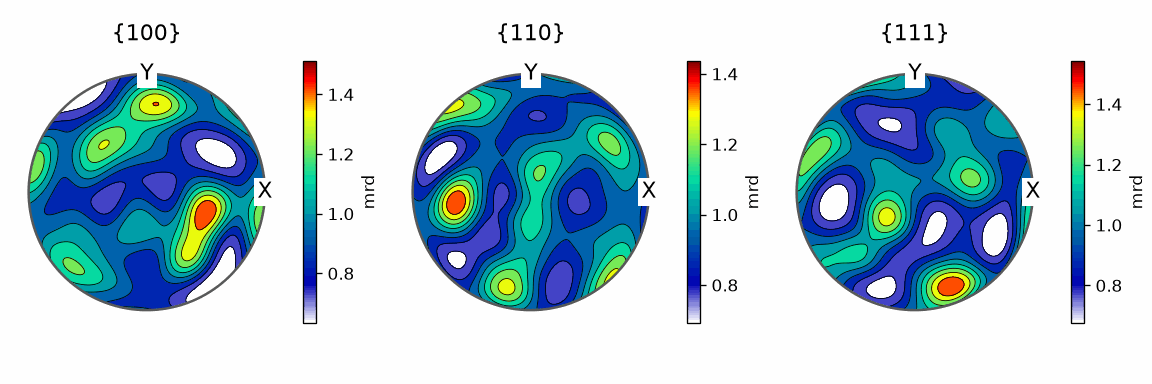
Nothing about the specimen changed between the two figures, and nothing about the measurements did either. The dozens of 4 mrd spots have become a gentle undulation reaching 1.5 mrd, because one hidden parameter was given a different value. A number read off the first figure is therefore a statement about the halfwidth as much as about the copper.

Estimate the density explicitly

calcDensity performs the same construction in orientation space and returns the result as an object. An orientation distribution function (ODF) is a density over the orientations of one phase, normalized so that a uniform texture is 1 mrd.

odf = calcDensity(ori, halfwidth=10 * degree)
odf

SO3FunHarmonic (Copper → y↑→x)
  bandwidth: 25
  mean     : 1

peakDensity = max(odf)[0]
peakDensity

3.7270

plotSection(odf, 'sigma', sections=6, contourf=True)
mtexColorbar(title='mrd')

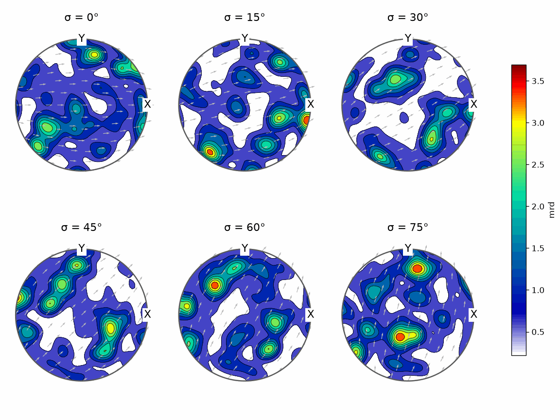
The maxima sit where the knots of the scatter plot were, and the highest reaches 3.7 mrd. Unlike the contoured pole figure, this estimate is a function that can be evaluated, integrated, and compared.

The contoured pole figure was the same estimate seen through one projection. Contouring poles with a given halfwidth reproduces the pole figure of the ODF estimated with that halfwidth exactly, because projecting the orientation-space kernel onto the sphere gives the kernel used there. What calcDensity adds is that the choice is visible and the result is kept.

The halfwidth is the decisive parameter

Estimate the same map with a sharper and a smoother kernel and collect the peak densities.

odfSharp = calcDensity(ori, halfwidth=4 * degree)
odfSmooth = calcDensity(ori, halfwidth=20 * degree)

halfwidthInDegree = [4, 10, 20]
peakMRD = [max(odfSharp)[0], max(odf)[0], max(odfSmooth)[0]]
for hw, p in zip(halfwidthInDegree, peakMRD):
  print(f'halfwidth {hw:2d} degree: peak {p:.4g} mrd')

halfwidth  4 degree: peak 37.26 mrd
halfwidth 10 degree: peak 3.727 mrd
halfwidth 20 degree: peak 1.449 mrd

A factor of five in halfwidth moves the peak by a factor of twenty five, from 37 mrd to 1.5 mrd. All three describe the same 16116 measurements, so at most one of them describes the copper.

Reconstruct the grains and plot the sharpest estimate with one marker per grain mean orientation on top of it. minPixel discards segmented regions below five pixels; Grain Reconstruction explains that choice.

grains = calcGrains(ebsd, minPixel=5)
copperGrains = grains['copper']
grainCount = len(copperGrains)
grainCount

368

plotSection(odfSharp, 'sigma', sections=6, contourf=True)
hold(True)
plotSection(copperGrains.meanOrientation, 'sigma', sections=6, markerSize=3, all=True, markerFaceColor='none', markerEdgeColor='k')
hold(False)

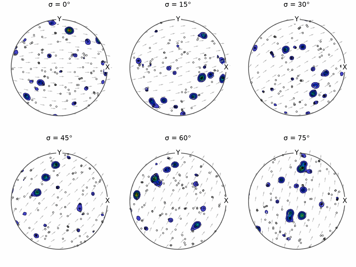
Every spike sits on a black marker, and the sections are white between them. With a 4 degree kernel the estimate is a picture of the few hundred grains rather than of a texture, and its 37 mrd maximum lies a fraction of a degree from the mean orientation of the largest grain. One well-measured grain has become a texture component.

Every ODF averages 1 mrd over orientation space, since that is what the normalization means. Ask this one for its average at the grain mean orientations alone.

sharpAtGrainMeans = np.mean(odfSharp.eval(copperGrains.meanOrientation))
sharpAtGrainMeans

5.7919

The grains carry about six times the average density, which is where the spikes came from. The opposite extreme fails the other way round.

plotSection(odfSmooth, 'sigma', sections=6, contourf=True)
mtexColorbar(title='mrd')

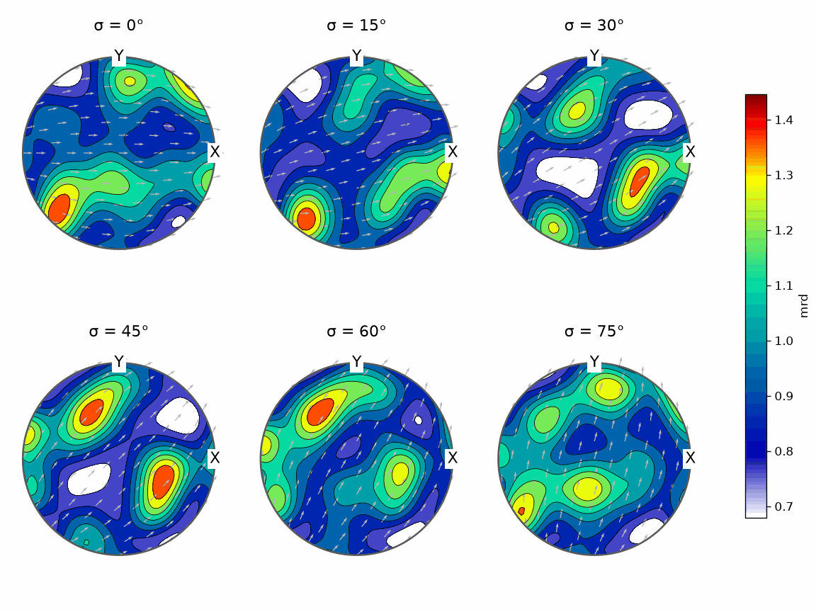
The whole function now lies between 0.7 and 1.5 mrd, and neighbouring maxima of the previous figures have merged into single broad hills. A genuine sharp component would be flattened the same way, so this estimate cannot distinguish a weak texture from a smeared strong one.

Between those extremes there is no value that is right in general. A halfwidth that is too small reproduces the individual grains, one that is too large erases the features worth reporting, and which of the two errors matters depends on how representative the map is for the whole specimen. A map holding a few hundred grains cannot support a sharp ODF, however many pixels it has.

Letting the data choose the halfwidth

calcKernel with method='KLCV', MATLAB’s default, selects a halfwidth by cross-validation. It leaves one orientation out, estimates a density from the rest, and scores how well that estimate predicts the omitted one. The halfwidth with the best score over the whole sample wins. No model of the texture is needed, only the sample.

The orientations of a map carry the mark notIID, since neighbouring pixels are not independent draws, and calcKernel refuses them. To see what cross-validation makes of the pixels anyway, clear the mark on a copy.

oriPixels = ori.copy()
oriPixels.notIID = False
psiPixel = calcKernel(oriPixels, method='KLCV')
pixelHalfwidth = psiPixel.halfwidth() / degree
pixelHalfwidth

2.7377

The pixel list returns 2.7 degrees, the regime that reproduces the grains. The reason is an assumption, not a bug: cross-validation treats the observations as independent draws. Neighbouring pixels of one grain are near copies of each other, so an omitted pixel is predicted almost perfectly by the pixels beside it, and the score keeps improving as the kernel narrows.

Give the selection one orientation per grain instead. Grain means are not perfectly independent either, but they no longer contain the same crystal measured hundreds of times.

psiGrain = calcKernel(copperGrains.meanOrientation, method='KLCV')
grainHalfwidth = psiGrain.halfwidth() / degree
grainHalfwidth

4.7247

The grain means return 4.7 degrees. The two other methods offered by calcKernel read the same orientations quite differently.

psiThumb = calcKernel(copperGrains.meanOrientation, method='RuleOfThumb')
psiMagic = calcKernel(copperGrains.meanOrientation, method='magicRule')

for name, psi in [('KLCV', psiGrain), ('RuleOfThumb', psiThumb), ('magicRule', psiMagic)]:
  print(f'{name:12s} selected halfwidth {psi.halfwidth() / degree:.4g} degree')

KLCV         selected halfwidth 4.725 degree
RuleOfThumb  selected halfwidth 14.31 degree
magicRule    selected halfwidth 15.02 degree

Cross-validation asks for 4.7 degrees while the two rules ask for about 15, and that spread is the useful result. The selected 4.7 degrees is barely above the 4 degrees of the spiky figure, so even grain means put the automatic choice in the regime where single grains are visible.

The methods answer different questions. Cross-validation asks which halfwidth describes this sample best, which is the right question only when the sample is the specimen. The two rules read only the number of orientations and the symmetry, and a few hundred orientations do not buy a sharp estimate. Optimal Kernel Selection compares the three methods against a known model ODF, where the best halfwidth can be measured rather than argued.

Selecting from the pixels and their grains

Two further methods of calcKernel estimate the error of the density itself, from the harmonic coefficients of the sample. 'UCV' aims at the halfwidth of least integrated squared error, 'conservative' at one that is at least as wide. Both accept the map once its grains are computed: the pixels are then compared only across groups of grains that share no grain, so the near copies inside a grain drop out without discarding a pixel. calcGrains above left the grain ids on ebsd.

rng = np.random.default_rng(0)
copperPixels = ebsd['copper']
psiUCV = calcKernel(copperPixels, method='UCV', rng=rng)
psiConservative = calcKernel(copperPixels, method='conservative', rng=rng)

for name, psi in [('UCV', psiUCV), ('conservative', psiConservative)]:
  print(f'{name:12s} selected halfwidth {psi.halfwidth() / degree:.4g} degree')

UCV          selected halfwidth 7.488 degree
conservative selected halfwidth 28.03 degree

UCV asks for 9.7 degrees and the conservative rule for 27, and again the spread is the result. The grains are few and of very different sizes: weighted by their area, the map carries as much information as about a hundred equally sized grains. UCV alone would follow the sample down to the narrowest kernel its harmonic bandwidth resolves; its noise floor stops it where the sampling noise of a hundred grains would raise bumps above a fifth of the maximum. The conservative rule finds the texture’s harmonic energies only loosely bounded and stays wide. Close to MATLAB’s 10 degrees, then, but for a reason that can be stated.

What one observation stands for

The halfwidth settles how far each observation spreads. Which observations enter the sum is a separate question with three common answers. All estimates so far used one observation per pixel; the other two put one observation per grain, with and without an area weight.

odfEqualGrain = calcDensity(copperGrains.meanOrientation, halfwidth=10 * degree)
odfAreaGrain = calcDensity(copperGrains.meanOrientation, weights=copperGrains.area, halfwidth=10 * degree)

for name, f in [('every pixel', odf), ('every grain', odfEqualGrain), ('grain means by area', odfAreaGrain)]:
  print(f'{name:22s} peak {max(f)[0]:.4g} mrd, distance to the pixel ODF {calcError(odf, f):.4g}')

every pixel            peak 3.727 mrd, distance to the pixel ODF 0
every grain            peak 2.536 mrd, distance to the pixel ODF 0.1606
grain means by area    peak 3.976 mrd, distance to the pixel ODF 0.0164

On a regular scan, one pixel per measurement weights each orientation by the area it covers. Grain means with equal weights describe the population of segmented grains, where a five-pixel grain counts as much as a several-hundred-pixel one; its peak is the weakest of the three. Weighting the grain means by grain area restores area weighting and comes back close to the pixel estimate: calcError measures about 0.02 against it, where equal grain weights measure 0.16.

The two grain-based estimates share a cost that the table does not show. Each grain enters as a single orientation, so the orientation spread inside it is discarded entirely.

meanSpread = np.mean(copperGrains.GOS) / degree
meanSpread

1.0834

maxSpread = np.max(copperGrains.GOS) / degree
maxSpread

6.9751

In this recrystallized copper the mean spread within a grain is about a degree and at most seven degrees, well below any halfwidth considered here, so little is lost. In deformed material the spread inside one grain reaches tens of degrees and carries much of the texture. There a grain-mean ODF is not a smoothed version of the pixel ODF but a different quantity, and a map with few grains rests the whole estimate on very few numbers.

A practical division of labour follows from the two sections: select the halfwidth from grain means, which are approximately independent, or from the pixels together with their grain ids, and estimate the density from the pixels, which carry the area and the intragranular spread.

Whatever the choice, state it. An area fraction measured in a section is not automatically a bulk volume fraction; that step needs sampling and stereological assumptions of its own.

Finally, do not estimate a density from a densified or interpolated copy of a map. Repeated cells are not new measurements and would take extra statistical weight. Regridding and Interpolation explains that distinction.

The definition

Let \(\psi : \mathrm{SO}(3) \to \mathbf{R}\) be a radially symmetric, unimodal kernel. Let the orientations \(o_1,o_2,\ldots,o_M\) carry non-negative weights \(w_1,w_2,\ldots,w_M\). The weighted kernel density estimator is

Each observation contributes one copy of \(\psi\) centred on itself, and its weight sets how much mass that copy carries. The halfwidth of \(\psi\) is the only smoothing parameter.

The formula suppresses symmetry notation for readability. MTEX accounts for the symmetry-equivalent representatives carried by each orientation. Different phases generally carry different crystal symmetries, which is why an EBSD-derived ODF is estimated from one selected phase at a time. Kernel Functions on SO(3) compares the available kernel families, and Density Estimation develops the same estimator for real numbers and for directions.

References

• R. Hielscher, Kernel density estimation on the rotation group and its application to crystallographic texture analysis, Journal of Multivariate Analysis 119 (2013), 119–143, gives the estimator used by calcDensity, the cross-validation rule used by calcKernel, and the fast algorithms behind both. The 'UCV' and 'conservative' rules are described in Optimal Kernel Selection.
• H.-J. Bunge, Texture Analysis in Materials Science: Mathematical Methods, Butterworths, English ed., 1982, develops orientation distributions, their symmetry, and the mrd normalization used throughout this page.
• J. Galán López and L. A. I. Kestens, A multivariate grain size and orientation distribution function: derivation from electron backscatter diffraction data and applications, Journal of Applied Crystallography 54 (2021), 148–162, treats grain frequency, grain size, and orientation as linked distributions rather than interchangeable weights.

Next

Optimal Kernel Selection examines the selection methods behind calcKernel where the true density is known. ODF Analysis explains what else an ODF can be asked, and ODF Plots and ODF Characteristics visualize and quantify the estimate.

@article{bachmann2010mtex,
  author  = {F. Bachmann and R. Hielscher and H. Schaeben},
  title   = {Texture Analysis with MTEX - Free and Open Source Software Toolbox},
  journal = {Solid State Phenomena},
  volume  = {160},
  pages   = {63-68},
  year    = {2010},
  doi     = {10.4028/www.scientific.net/SSP.160.63},
  url     = {https://doi.org/10.4028/www.scientific.net/SSP.160.63}
}