Optimal Kernel Selection

Density Estimation showed that kernel width decides which features survive smoothing. A width that is too small leaves oscillations and sharp peaks at individual observations. A width that is too large erases genuine features of the unknown density.

There is no universally optimal halfwidth. The useful value depends on both the number of independent observations and the smoothness of the unknown density. This page compares the selection methods provided by calcKernel and shows how to check their choices against a known model.

import matplotlib.pyplot as plt
import numpy as np

from mtex import *

plottingConvention.default('y↑→x')
rng = np.random.default_rng(1)

Build a model with several kinds of structure

The original example described the following crystal symmetry as cubic. Point group 321 is trigonal, so the code and its resulting fundamental region must be read as a trigonal example.

cs = crystalFrame('321')

Combine a uniform background, one localized component, and one fibre. Their coefficients sum to one, so modelODF remains normalized.

modelODF = (0.25 * uniformODF(cs)
            + 0.25 * unimodalODF(orientation.byEuler(np.array([35, 45, 0]) * degree, cs))
            + 0.5 * fibreODF(Miller(7, -1, 10, cs), vector3d(7, -5, 11), halfwidth=10 * degree))

plot(modelODF, 'sigma', sections=6)
mtexColorbar(title='mrd')

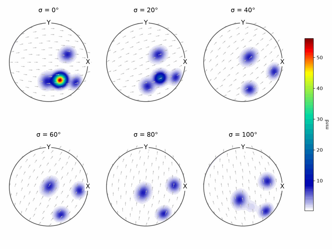
The sections contain a localized maximum and an elongated fibre feature above a non-zero background. A useful selected kernel should retain both shapes without turning finite-sample noise into new maxima.

Select a kernel from sampled orientations

Draw 10000 orientations from the model. The random generator seeded at the top of the page makes the sample and every reported result reproducible.

ori = discreteSample(modelODF, 10000, rng=rng)
sampleCount = len(ori)
sampleCount

10000

MATLAB’s calcKernel uses Kullback–Leibler cross-validation (KLCV) when no method is named; the port’s default is 'UCV', described below, so KLCV is named here. It returns a de la Vallée Poussin kernel rather than an ODF.

psi = calcKernel(ori, method='KLCV', rng=rng)
psi

SO3DeLaValleePoussinKernel
  bandwidth: 35
  halfwidth: 7.14°

selectedHalfwidth = psi.halfwidth() / degree
selectedHalfwidth

7.1380

Pass that kernel to calcDensity. The same psi can therefore be reused for another sample that represents the same population and sampling process.

reconstructedODF = calcDensity(ori, kernel=psi)
reconstructionError = calcError(reconstructedODF, modelODF, resolution=5 * degree)
reconstructionError

0.1390

plot(reconstructedODF, 'sigma', sections=6)
mtexColorbar(title='mrd')

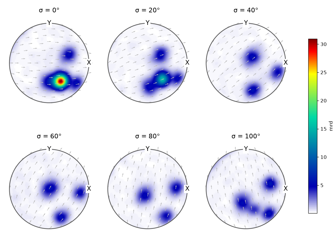
Compare these sections with the model above. The localized maximum and the fibre remain in the same places, while their contours are not identical because only a finite random sample was reconstructed.

reconstructionError compares density values over orientation space. It is not an angular error and must not be labelled in degrees.

Select from the error of the density

Two further methods judge a candidate kernel by the error of the density it produces. 'UCV' (unbiased cross-validation), the port’s default, estimates the integrated squared error of every candidate from the harmonic coefficients of the sample and takes the halfwidth where it is least. 'conservative' replaces the texture’s harmonic energies by lower confidence bounds and ignores the harmonic degrees it cannot resolve; the halfwidth it returns is then at least as wide as the one of least error. Both are bounded below by a noise floor: no halfwidth so narrow that the sampling noise could raise bumps above a fifth of the estimate’s maximum, with noiseFloor=False to switch it off. Both cost about one harmonic transform of the sample, under a second for a million orientations. They use their own random generator here, which splits the sample into the parts it compares.

rngSelect = np.random.default_rng(2)
for m in ['UCV', 'conservative']:
  psiM = calcKernel(ori, method=m, rng=rngSelect)
  errorM = calcError(calcDensity(ori, kernel=psiM), modelODF, resolution=5 * degree)
  print(f'{m:12s} halfwidth {psiM.halfwidth() / degree:.3g} degree, error {errorM:.3g}')

UCV          halfwidth 4.07 degree, error 0.131
conservative halfwidth 4.07 degree, error 0.131

Both ask for 4.1 degrees against the 7.1 degrees of KLCV above, and their error, 0.131, lies below KLCV’s 0.139. With 10000 orientations the harmonic energies of this texture are resolved well enough that the conservative bound and the unbiased estimate agree.

What the methods use

The method names are sometimes described as flags in older material. The current interface passes each name as the value of method.

Older descriptions say that 'RuleOfThumb' uses the variance of the orientations to estimate smoothness. The current implementation instead uses a quantile of nearest-neighbour angular distances, with a lower halfwidth limit of 2 degrees.

KLCV evaluates how well kernels centred on the other orientations predict each omitted orientation. The samplingSize option limits how many observations contribute to that score. It reduces computation, but it does not create an independent validation dataset.

Compare the methods on the same samples

The full scaling experiment associated with this page uses 10, 100, …, 1000000 orientations. That run is appropriate for an attended benchmark, not an executable documentation page. Uncomment the alternative sampleSize line when that full study is intended.

sampleSize = [30, 100, 300, 1000]
# sampleSize = 10 ** np.arange(1, 7)   # full study: 10 through 1000000

method = ['KLCV', 'RuleOfThumb', 'magicRule', 'UCV', 'conservative']
halfwidthInDegree = np.zeros((len(sampleSize), len(method)))
estimationError = np.zeros((len(sampleSize), len(method)))

for i, n in enumerate(sampleSize):
  oriTrial = discreteSample(modelODF, n, rng=rng)
  for j, m in enumerate(method):
    psiTrial = calcKernel(oriTrial, method=m, samplingSize=1000, rng=rngSelect if m in ('UCV', 'conservative') else rng)
    trialODF = calcDensity(oriTrial, kernel=psiTrial)
    halfwidthInDegree[i, j] = psiTrial.halfwidth() / degree
    estimationError[i, j] = calcError(trialODF, modelODF, resolution=7.5 * degree)

rowName = [f'N_{n}' for n in sampleSize]
print('halfwidthTable')
print(f"{'':8}" + ''.join(f'{m:>13}' for m in method))
for r, row in zip(rowName, halfwidthInDegree):
  print(f'{r:8}' + ''.join(f'{v:13.3f}' for v in row))
print('\nerrorTable')
print(f"{'':8}" + ''.join(f'{m:>13}' for m in method))
for r, row in zip(rowName, estimationError):
  print(f'{r:8}' + ''.join(f'{v:13.5f}' for v in row))

halfwidthTable
                 KLCV  RuleOfThumb    magicRule          UCV conservative
N_30           23.811       55.110       26.117       38.020       40.000
N_100          11.906       33.501       22.018       12.442       16.037
N_300          11.906       24.646       18.836       11.240       11.240
N_1000          9.449       16.983       15.870        6.112        6.112

errorTable
                 KLCV  RuleOfThumb    magicRule          UCV conservative
N_30          0.44184      0.54391      0.45433      0.50625      0.51213
N_100         0.29798      0.46635      0.39014      0.30117      0.33489
N_300         0.28499      0.42540      0.36964      0.27891      0.27891
N_1000        0.21704      0.33845      0.32227      0.22162      0.22162

Read each row as one random sample tested five ways. This controls the sample-to-sample variation when comparing methods within a row. One draw at each size is a demonstration, not evidence that one method is always best.

With 30 orientations the two new rules return nearly their widest candidates, 38 and 40 degrees: the noise floor finds that nothing narrower would stand out of the sampling noise, and their error is the price of that caution. From 300 orientations on they agree, and at 1000 orientations they ask for 6.1 degrees where KLCV asks for 9.4, at nearly the same error.

plt.figure()
plt.loglog(sampleSize, estimationError, 'o-', linewidth=2)
plt.legend(method, loc='best')
plt.xlabel('number of orientations')
plt.ylabel('ODF estimation error')
plt.grid(True, which='both')

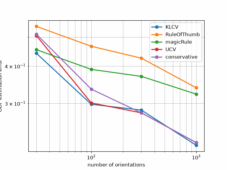
The curves compare density-space error, with smaller values indicating a closer reconstruction. Their differences show that kernel selection is part of the statistical model rather than a display preference.

Before trusting an automatic halfwidth

Automatic selection assumes that the input orientations represent the intended population. Neighbouring pixels in one EBSD grain are strongly correlated, so treating every pixel as independent can select a kernel that follows intragranular scatter. The orientations of a map therefore carry the mark notIID, and calcKernel refuses them. 'UCV' and 'conservative' accept them with the grain id of every pixel, groups=ebsd.grainId, or the map itself once its grains are computed; they then compare only parts of the sample that share no grain. Otherwise use grain means to select the kernel when grains are the independent sampling units.

Weighting answers a separate question. After selecting a kernel from grain means, an area-based ODF may still use pixels or grain-area weights. ODF Estimation from EBSD Data works through that choice.

Also inspect the selected halfwidth and the reconstructed plots. A value at the edge of the tested candidate range, or peaks supported by only one or two observations, is a reason to test nearby kernels manually.

The maths behind the sample-size rule

For the de la Vallée Poussin kernel, 'magicRule' sets the concentration parameter \(\kappa\) proportional to \(N^{2/7}\). The kernel halfwidth then behaves approximately as

The rule therefore narrows the kernel as the sample grows. It cannot use the unknown density’s feature sizes, which is why it is conservative. Rule-of-thumb and cross-validation methods use the observations to add information about those scales.

The maths behind UCV and the conservative rule

Write the density in harmonics orthonormal for the uniform distribution, \(f = 1 + \sum_{\ell \ge 1} f_\ell\), with the degree energies \(A_\ell = \|f_\ell\|^2\). A radial kernel multiplies degree \(\ell\) by a factor \(b_\ell\) that falls as the halfwidth grows. For \(N\) independent orientations the mean integrated squared error is exactly

where \(d_\ell\) is the dimension of degree \(\ell\) reduced by the crystal and specimen symmetry. 'UCV' inserts unbiased estimates of \(A_\ell\), obtained from products of disjoint parts of the sample, and minimises over the candidates. 'conservative' inserts lower confidence bounds and sets the unresolved high degrees to zero. Lowering the energies can only move the minimiser to a wider kernel, so the choice is at least the halfwidth of least error whenever the bounds hold. Splitting a map into parts that share no grain keeps the estimates unbiased when pixels of one grain are correlated.

The noise floor looks at the estimate itself. At an orientation where the smoothed density is \(y\), the estimate is a sum of \(N\) independent terms, none larger than \(\psi(0)/N\), with variance \(y\,\|\psi\|^2/N\). Bennett’s inequality bounds its deviation at every one of the independent kernel footprints of orientation space, and the floor is the smallest halfwidth at which that bound stays below a fifth of the estimate’s maximum plus half the local density.

References

• R. Hielscher, Kernel density estimation on the rotation group and its application to crystallographic texture analysis, Journal of Multivariate Analysis 119 (2013), 119–143, derives the orientation-space estimator, asymptotic halfwidth rules, and fast algorithms used for large orientation samples.

Next

Clustering replaces a continuous density by discrete groups of nearby orientations. Use it when group membership is the goal rather than estimating how probability varies through orientation space.

@article{bachmann2010mtex,
  author  = {F. Bachmann and R. Hielscher and H. Schaeben},
  title   = {Texture Analysis with MTEX - Free and Open Source Software Toolbox},
  journal = {Solid State Phenomena},
  volume  = {160},
  pages   = {63-68},
  year    = {2010},
  doi     = {10.4028/www.scientific.net/SSP.160.63},
  url     = {https://doi.org/10.4028/www.scientific.net/SSP.160.63}
}