Regridding and Interpolating EBSD Data

An EBSD map stores one measurement at each acquired position. Denoising changes noisy orientations without moving those positions. Filling Missing Data supplies values at missing positions while leaving the measurement grid unchanged.

This page considers the other operation: reading the map at positions that were not measured, then sampling it on a different grid. MTEX uses nearest neighbours for this operation. It does not average orientations.

The examples assume basic EBSD selection and the distinction between a list and a gridded EBSD map.

import matplotlib.pyplot as plt

from mtex import *

plottingConvention.default('y↑→x')
ebsd = mtexdata('twins')

Reading the Map at One Point

interp evaluates a map at arbitrary coordinates. It works with a plain EBSD list, a phase subset, and a rotated or sheared map. The imported map in this example happens to be a square grid.

x = 30.5
y = 5.5

plot(ebsd, ebsd.orientations)
hold(True)
plt.plot(x, y, 'ko', markerfacecolor='w', markersize=7)
hold(False)

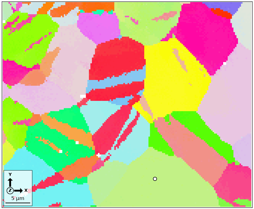
The marker identifies the requested position. It lies between the centres of the coloured source pixels, so the result must be sampled from one of them.

e1 = interp(ebsd, x, y)
e1

EBSD (y↑→x)
  size: 1
  Phase  Orientations  Mineral    Color         Symmetry  Crystal reference frame
  1      1 (100%)      Magnesium  LightSkyBlue  6/mmm     Magnesium
  Id  Phase             orientation  bands   bc   bs  error  mad
   0      1  (162.9°,111.9°,306.1°)     10  160  255      0  0.4
  scan unit: um
  X × Y    : [30.5 → 30.5] × [5.5 → 5.5]

The summary shows a new, one-entry EBSD variable at the requested position. MTEX finds the nearest source measurement and copies its phase, orientation, and per-pixel properties.

The query is accepted only when the nearest measurement is no farther away than the furthest corner of ebsd.unitCell. This circular distance cutoff is not a polygon-containment test. A point beyond that reach returns as notIndexed instead of being extrapolated, whether it is outside the map or sufficiently far inside a hole.

The 'xy' selector also finds the nearest source measurement.

e2 = ebsd['xy', x, y]
e2

EBSD (y↑→x)
  size: 1
  Phase  Orientations  Mineral    Color         Symmetry  Crystal reference frame
  1      1 (100%)      Magnesium  LightSkyBlue  6/mmm     Magnesium
    Id  Phase             orientation  bands   bc   bs  error  mad
  3108      1  (162.8°,112.1°,186.1°)     10  160  255      0  0.4
  scan unit     : um
  X × Y         : [30.6 → 30.6] × [5.4 → 5.4]
  square lattice: spacing 0.3

For this point, both commands therefore report the same orientation.

angle(e1.orientations, e2.orientations) / degree

array([0.1268])

The zero-degree result confirms the match. The two EBSD summaries expose the important difference: e2 retains the source position and id, whereas e1 sits at the requested position and receives a new id.

With a list of query positions, interp returns one new entry per query in the same order. That behavior makes resampling possible; 'xy' remains a selector for original measurements.

Resampling onto a Different Grid

A unit cell describes the shape and scale of a grid. gridify derives its cell-to-cell translations, builds a lattice over the map extent, and reads the nearest measurement at the new positions. Here the unit cell is twice as large and rotated by 45 degrees.

# unit cell of twice the size, rotated by 45 degrees
uC = rotate(2 * ebsd.unitCell, 45 * degree)

# resample the map on the new lattice
ebsdNewGrid = gridify(ebsd, unitCell=uC)
ebsdNewGrid

EBSD (y↑→x)
  size: 108 × 109 grid
  Phase  Orientations  Mineral     Color         Symmetry  Crystal reference frame
  0      6059 (51%)    notIndexed
  1      5713 (49%)    Magnesium   LightSkyBlue  6/mmm     Magnesium
  properties    : bands, bc, bs, error, mad
  scan unit     : um
  X × Y         : [-20.79 → 70.43] × [-25.03 → 66.19]
  square lattice: spacing 0.6

# plot only cells that received source data
plot(ebsdNewGrid['indexed'], ebsdNewGrid['indexed'].orientations)
ext = ebsd.extent()
plt.xlim(ext[0], ext[1])
plt.ylim(ext[2], ext[3])

(0.0, 40.8)

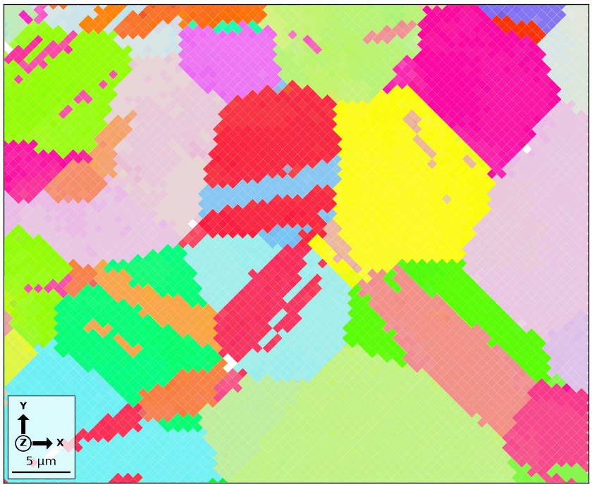
Compare this figure with the first map. The orientation regions occupy the same specimen positions, but their pixels are now coarser and tilted. The orientations themselves have not been rotated. The specimen’s grains also occupy the same physical regions; only their rasterized outlines have changed.

The summary reports a 108 by 109 matrix. A tilted lattice needs a larger rectangular matrix to cover the source extent, so its corner cells project beyond the map. Fewer than half of the cells are indexed, which is why the plot excludes notIndexed cells.

From a Hexagonal to a Square Grid

A custom unit cell can also change the grid type. The ferrite data was measured on a hexagonal grid.

plottingConvention.default('y↓→x')
ebsd = mtexdata('ferrite')

hexGridSize = ebsd.shape
hexGridSize

(270, 234)

plot(ebsd[0:50, 0:100], ebsd[0:50, 0:100].orientations)

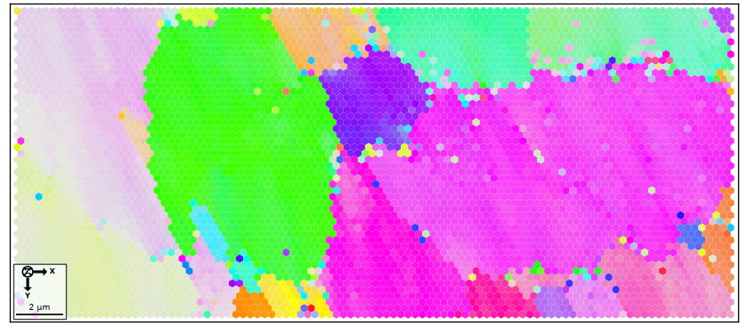
The staggered pixel rows reveal the hexagonal sampling lattice. Their orientations are measurements; the next figure only redraws those values on a different lattice.

A square cell with half the measurement spacing gives a drawing grid fine enough to distinguish neighbouring source positions in this example. This smaller cell does not improve the map’s spatial resolution.

# define a square unit cell
squnitCell = ebsd.dPos / 4 * vector3d([-1, -1, 1, 1], [-1, 1, 1, -1], 0)

# resample on the square lattice
ebsdS = ebsd.gridify(unitCell=squnitCell)

squareGridSize = ebsdS.shape
squareGridSize

(808, 809)

plot(ebsdS[0:150, 0:350], ebsdS[0:150, 0:350].orientations)

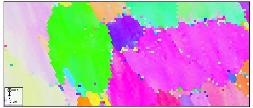
The result is a square grid with 808 by 809 cells in place of the 270 by 234 hexagonal cells, about ten times as many. The stepped colour regions show that each new cell repeats its nearest hexagonal measurement. No orientation was invented on the way.

What Regridding Does Not Change

Resampling changes the array size and pixel outlines, not the acquisition step or the spatial resolution of the experiment. Repeated cells are not independent measurements. Keep the original map for quantitative counts, orientation statistics, and grain-size measurements unless the analysis explicitly requires a new raster.

Every copied quality value still describes the original diffraction pattern. It is not evidence that a pattern was acquired at the new cell. Use Filling Missing Data to recover orientations at missing positions, or Denoising to reduce orientation noise. Neither task is performed by interp.

Further Reading

• R. C. Staunton, Hexagonal Sampling in Image Processing, Advances in Imaging and Electron Physics 107, 231–307 (1999), reviews the geometric consequences of converting between hexagonal and square sampling lattices.
• F. J. Humphreys, Review: Grain and subgrain characterisation by electron backscatter diffraction, Journal of Materials Science 36, 3833–3854 (2001), quantifies how EBSD step size limits grain-size measurements.
• ISO 13067:2020, Microbeam analysis - Electron backscatter diffraction - Measurement of average grain size, defines EBSD grain-size measurement on two-dimensional sections. Consult it before using a resampled raster for grain statistics.

Next

ODF Estimation turns measured map orientations into an orientation distribution function. Use the measured map rather than a densified copy so repeated cells do not acquire extra statistical weight.

@article{bachmann2010mtex,
  author  = {F. Bachmann and R. Hielscher and H. Schaeben},
  title   = {Texture Analysis with MTEX - Free and Open Source Software Toolbox},
  journal = {Solid State Phenomena},
  volume  = {160},
  pages   = {63-68},
  year    = {2010},
  doi     = {10.4028/www.scientific.net/SSP.160.63},
  url     = {https://doi.org/10.4028/www.scientific.net/SSP.160.63}
}