download as script · edit page

Most EBSD maps are measured on a square or hexagonal scan lattice. By default, EBSD.load keeps that structure: it returns a map on its square or hexagonal grid whenever every measurement fits on one lattice. Otherwise it keeps the measurements as a plain EBSD list and explains why.

This page assumes basic EBSD selection and plotting. See Select by Index first if row and column indexing is unfamiliar.

A scan lattice, a matrix layout, and a reference frame answer different questions. The lattice says which measurements are neighbours. The layout says which specimen directions the matrix indices follow. The reference frame says which axes the positions and orientations are expressed in.

import numpy as np

from mtex import *

plottingConvention.default('y↑→x')
ebsd = mtexdata('twins')
ebsd

EBSD (y↑→x)
  size: 137 × 167 grid
  Phase  Orientations  Mineral     Color         Symmetry  Crystal reference frame
  0      46 (0.2%)     notIndexed
  1      22833 (100%)  Magnesium   LightSkyBlue  6/mmm     Magnesium
  properties    : bands, bc, bs, error, mad
  scan unit     : um
  X × Y         : [0 → 49.8] × [0 → 40.8]
  square lattice: spacing 0.3

The summary identifies ebsd as a square grid. Its 22879 measurements form a 137 by 167 matrix, with one entry per scan position. Apart from its matrix shape, it behaves like any other EBSD variable.

plot(ebsd['Magnesium'], ebsd['Magnesium'].orientations)

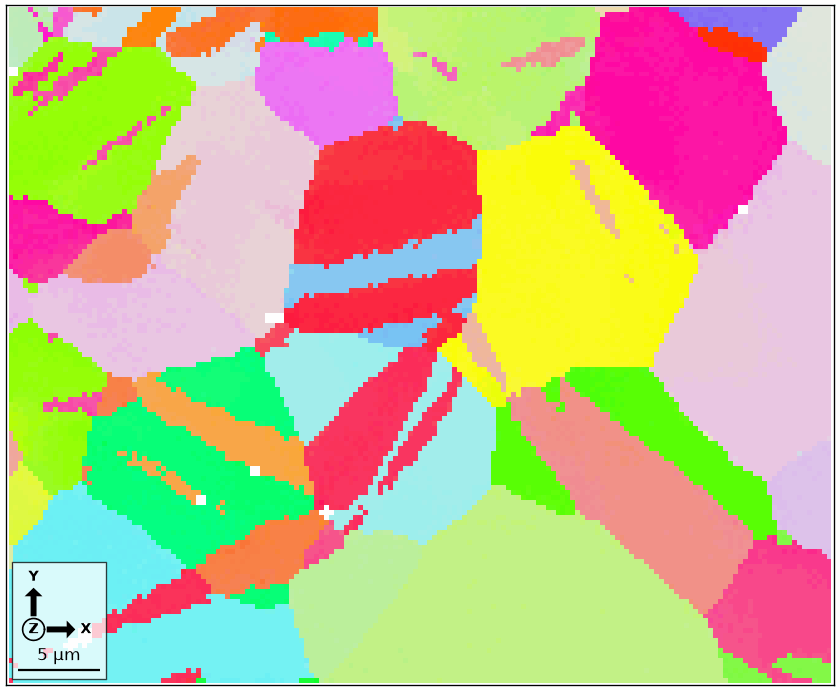
The rectangular outline follows the square measurement grid. The four corners of one pixel give the same information directly.

ebsd.unitCell

vector3d (y↑→x)
  size: 4
      x      y  z
   0.15   0.15  0
  -0.15   0.15  0
  -0.15  -0.15  0
   0.15  -0.15  0

What a Grid Is Good For

Per-pixel data can be handed to image-processing and registration tools as a matrix, and ebsd[i, j] addresses one scan position.
Plotting and denoising are considerably faster because the raster does not have to be reconstructed.

Matrix indexing means what it says. The measurement in row 49 and column 99, counted from zero, is

ebsd[49, 99]

EBSD (y↑→x)
  size: 1
  Phase  Orientations  Mineral    Color         Symmetry  Crystal reference frame
  1      1 (100%)      Magnesium  LightSkyBlue  6/mmm     Magnesium
    Id  Phase             orientation  bands   bc   bs  error  mad
  8282      1  (155.8°,100.6°,239.3°)     10  149  133      0  0.7
  scan unit     : um
  X × Y         : [29.7 → 29.7] × [14.7 → 14.7]
  square lattice: spacing 0.3

In the default layout, the first matrix dimension follows the grid direction closest to y. The second follows the direction closest to x. Both indices advance towards increasing coordinates. Thus ebsd[0, 0] is the corner with the smallest coordinates, and ebsd[i, j] is the j-th pixel in the i-th scan row.

This layout belongs to the map, not to the file traversal order. It is the same whichever corner the acquisition started from.

A stored matrix is not required nearly as often as it once was. The orientation gradient, curvature, GND, and fill operate on the virtual lattice derived by lattice. They also work on plain lists, phase subsets, and arbitrarily aligned maps.

Choosing the Layout

A matrix is useful for image processing only when it is stored the same way round as the image. A forescatter or BSE image follows the order in which its detector wrote the pixels. That order need not match the map. Maps and Images compares a real map with SEM images of the same area.

'columnMajor' and 'rowMajor' are the two layouts aligned with x and y. Both are gridLayout objects. A layout names the row direction first, in the same order as the shape of the array. Suppose an image’s rows run against x and its columns run along y, as for a detector mounted a quarter turn from the scan.

gL = gridLayout(-xvector, yvector)

Handing that layout to gridify changes the matrix shape and ordering.

ebsdI = gridify(ebsd, gL)
ebsdI

EBSD (y↑→x)
  size: 167 × 137 grid
  Phase  Orientations  Mineral     Color         Symmetry  Crystal reference frame
  0      46 (0.2%)     notIndexed
  1      22833 (100%)  Magnesium   LightSkyBlue  6/mmm     Magnesium
  properties    : bands, bc, bs, error, mad
  scan unit     : um
  X × Y         : [0 → 49.8] × [0 → 40.8]
  square lattice: spacing 0.3

The map records the layout in which it is stored.

ebsdI.layout

gridLayout
  row: (-1, 0, 0)
  col: (0, 1, 0)

Every per-pixel property follows the same layout. For this pair of layouts, band contrast is related by a quarter turn.

np.array_equal(ebsdI.bc, np.rot90(ebsd.bc))

True

No value was resampled or invented. A transpose and flips are sufficient, so conversion back to the original layout is exact.

np.array_equal(gridify(ebsdI, ebsd.layout).bc, ebsd.bc)

True

Layout changes storage, not the specimen. The positions and orientations are unchanged, and the plotting convention still draws both maps in the same specimen frame.

newMtexFigure(layout=[1, 2])
plot(ebsd, ebsd.bc)
mtexColorMap('gray')
mtexTitle('columnMajor')
nextAxis()
plot(ebsdI, ebsdI.bc)
mtexColorMap('gray')
mtexTitle('row against x, column along y')

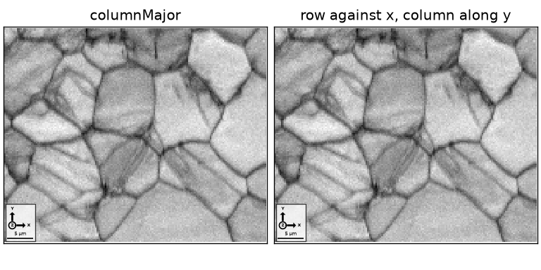
The same features occupy the same screen positions in both panels. Only the labels describe a different order in memory.

Data That Cannot Be Put on a Grid

A rectangular raster is faithful only when every measurement occupies a distinct site of one lattice. If two measurements land in the same cell, one would be lost. MTEX therefore keeps such data as a list and reports the problem rather than silently dropping a measurement.

ebsd = EBSD.load(mtexdatafile('eclogite'), eulerCorrection=rotation.byAxisAngle(zvector, 180 * degree))
ebsd

Warning: the measurements are not on a lattice; keeping the data as a list
EBSD (y↑→x)
  size: 617
  Phase  Orientations  Mineral                Color       Symmetry  Crystal reference frame
  0      4 (0.65%)     notIndexed
  4      165 (27%)     Garnet - (Mg,Ni)3Al2(  LightCoral  m-3m      Garnet - (Mg,Ni)3Al2(
  5      215 (35%)     Omphacite              DarkBlue    12/m1     Omphacite
  6      61 (9.9%)     Coesite                DarkGreen   12/m1     Coesite
  7      172 (28%)     Quartz-new             DarkRed     -3m1      Quartz-new
  properties: bands, bc, bs, error, mad
  scan unit : um
  X × Y     : [1.911 → 716.5] × [1.91 → 622.9]

The warning above says why the data stays a list. MTEX also keeps a list when the positions are too irregular to span a sensible raster. You may request a list independently of the data, either for one import,

ebsd = EBSD.load(fname, grid=False)

or for the whole session.

setMTEXpref('gridifyOnImport', False)

You may change representation later. ebsd.flatten() flattens a gridded map into a list, while gridify puts a list on its grid.

Selecting a Subset Drops the Matrix Shape

Selecting a phase, region, or indexed measurements usually leaves a shape that is not rectangular. The result is therefore a plain list, although every retained measurement still lies on the original lattice.

ebsd = mtexdata('twins')

ebsdMg = ebsd['Magnesium']
ebsdMg

EBSD (y↑→x)
  size: 22833
  Phase  Orientations  Mineral    Color         Symmetry  Crystal reference frame
  1      22833 (100%)  Magnesium  LightSkyBlue  6/mmm     Magnesium
  properties    : bands, bc, bs, error, mad
  scan unit     : um
  X × Y         : [0 → 49.8] × [0 → 40.8]
  square lattice: spacing 0.3

Reapplying gridify restores the matrix shape.

ebsdMg = ebsd['Magnesium'].gridify()
ebsdMg

EBSD (y↑→x)
  size: 137 × 167 grid
  Phase  Orientations  Mineral    Color         Symmetry  Crystal reference frame
  1      22833 (100%)  Magnesium  LightSkyBlue  6/mmm     Magnesium
  properties    : bands, bc, bs, error, mad
  scan unit     : um
  X × Y         : [0 → 49.8] × [0 → 40.8]
  square lattice: spacing 0.3

The variables ebsd and ebsdMg differ at the 46 positions that were not indexed. In ebsd those are real measurements in the separate 'notIndexed' phase: a diffraction pattern was recorded but could not be indexed. Selecting magnesium removes those measurements and creates gaps, meaning missing sites within scan lines.

After gridify, each gap is an empty lattice site in ebsdMg. Its orientation is NaN and its id lies beyond the ids of the parent map, because no selected measurement belongs there. It is not a notIndexed measurement.

[np.sum(ebsd.id >= ebsd.size), np.sum(ebsdMg.id >= ebsd.size)]

[0, 46]

The empty sites complete the rectangle. Row and column ranges can therefore select and plot a rectangular subregion.

plot(ebsdMg[49:100, 4:100], ebsdMg[49:100, 4:100].orientations)

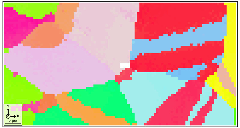
Gridding Reorders the Measurements

gridify does not preserve input order, and generally cannot. The layout fixes the first matrix dimension to y, whereas .ctf and .ang files usually write x fastest. Consequently, the k-th entry of the flattened grid is generally not line k of the input file.

Nothing is lost. The id of every measurement keeps its number in the imported list, the record MATLAB keeps as the property oldId. Its upper left corner shows consecutive ids running along matrix rows.

ebsd.id[0:3, 0:4]

array([[  0,   1,   2,   3],
       [167, 168, 169, 170],
       [334, 335, 336, 337]])

The index return_index=True adds, MATLAB’s second output of gridify, translates in the other direction. In particular, ebsdGrid.pos at newId returns the gridded positions in the order of the input list.

ebsdGrid, newId = gridify(ebsd.flatten(), return_index=True)

np.array_equal(ebsdGrid.pos.flatten()[newId].data, ebsd.flatten().pos.data)

True

This distinction matters only to code that depends on input order. Grain reconstruction does not: calcGrains returns the same grains from the list and from the map.

The Gradient

The orientation gradient, the incomplete Nye tensor, and the gradient form of the weighted Burgers vector are computed on the virtual lattice. They therefore do not require a stored matrix. The default integral form of the weighted Burgers vector is a raster algorithm and grids internally.

A grid does no harm, so this example continues with ebsdMg. The result has the same matrix shape as the map.

gradX = ebsdMg.gradientX()

plot(ebsdMg, norm(gradX))
setColorRange([0, 4 * degree])

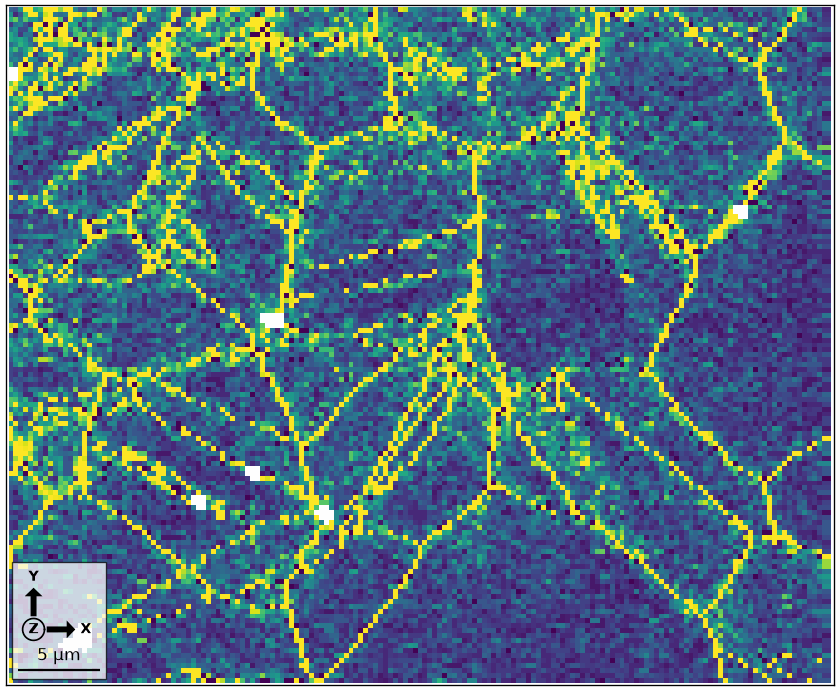
The colour field follows the same rectangular raster, including its empty sites. No separate gridding step was needed for the derivative itself.

Hexagonal Grids

The same principles apply to a hexagonal scan. MTEX imports it on its hexagonal grid and provides the same row and column indexing.

ebsd = mtexdata('copper')

grains = calcGrains(ebsd)

ebsd

EBSD (y↑→x)
  size: 136 × 119 grid
  Phase  Orientations  Mineral  Color         Symmetry  Crystal reference frame
  1      16116 (100%)  Copper   LightSkyBlue  m-3m      Copper
  properties : confidenceindex, extra1, extra2, extra3, extra4, fit, grainId, imagequality, semsignal
  scan unit  : um
  X × Y      : [0 → 590] × [0 → 584.6]
  hex lattice: spacing 5

plot(ebsd[0:20, 0:40], ebsd[0:20, 0:40].orientations, micronbar=False, edgeColor='black')

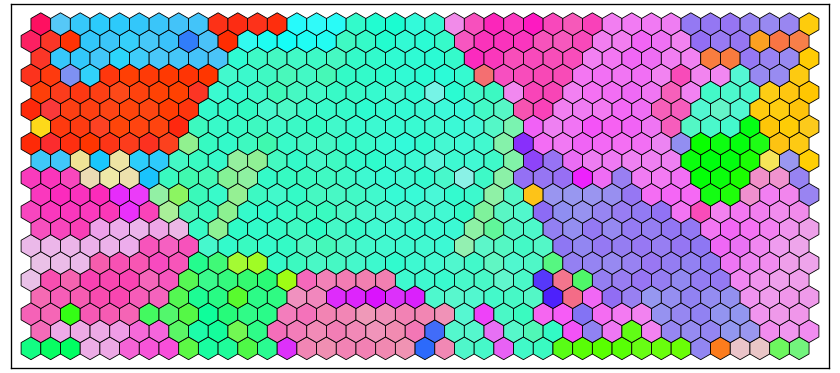
The black cell edges reveal the alternating half-step offset between scan rows. The matrix is rectangular even though its pixel footprints are hexagons.

Switching from a Hexagonal to a Square Grid

Some external image-processing tools require square pixels. Passing a square unitCell to gridify resamples the hexagonal measurements onto such a grid.

# define a square unit cell
unitCell = 2.5 * vector3d([-1, -1, 1, 1], [-1, 1, 1, -1], 0)

# use the square unit cell for gridify
ebsdS = ebsd.gridify(unitCell=unitCell)
ebsdS

EBSD (y↑→x)
  size: 118 × 119 grid
  Phase  Orientations  Mineral  Color         Symmetry  Crystal reference frame
  1      14042 (100%)  Copper   LightSkyBlue  m-3m      Copper
  properties    : confidenceindex, extra1, extra2, extra3, extra4, fit, grainId, imagequality, semsignal
  scan unit     : um
  X × Y         : [0 → 590] × [0 → 585]
  square lattice: spacing 5

# visualize the result
newMtexFigure(layout=[1, 2])
plot(ebsd, ebsd.orientations)
nextAxis()
plot(ebsdS, ebsdS.orientations)

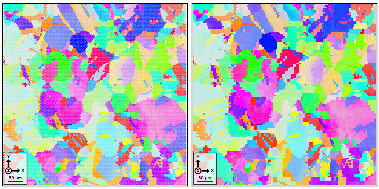
This operation differs fundamentally from restoring a map’s own lattice. The new grid sites do not coincide with the measured ones, so every site copies the values of the nearest measurement. The left panel shows the measured hexagons; the right shows the square pixels after resampling.

The square cell above has approximately the same size as the hexagonal one. Squares cannot reproduce hexagonal outlines, so grain boundaries in the right panel are visibly staircased. A smaller square cell reduces the size of the steps.

# a smaller unit cell
unitCell = 0.5 * vector3d([-1, -1, 1, 1], [-1, 1, 1, -1], 0)

# use the small square unit cell for gridify
ebsdS = ebsd.gridify(unitCell=unitCell)
ebsdS

EBSD (y↑→x)
  size: 586 × 591 grid
  Phase  Orientations   Mineral  Color         Symmetry  Crystal reference frame
  1      346326 (100%)  Copper   LightSkyBlue  m-3m      Copper
  properties    : confidenceindex, extra1, extra2, extra3, extra4, fit, grainId, imagequality, semsignal
  scan unit     : um
  X × Y         : [0 → 590] × [0 → 585]
  square lattice: spacing 1

plot(ebsdS, ebsdS.orientations)
hold(True)
plot(grains.boundary, lineWidth=2)
hold(False)

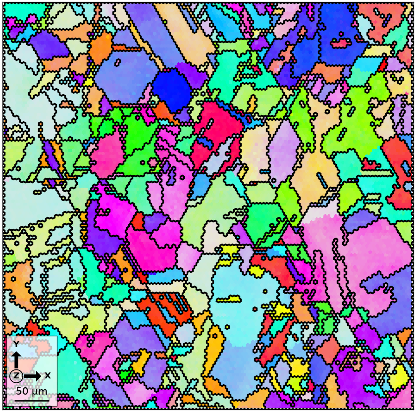
The smaller cells follow the original boundary more closely. They do not add spatial resolution: every new orientation still comes from a nearest measured hexagon. Regridding and Interpolation develops this distinction in detail.

Pixels that remain notIndexed correspond to measurements that were not indexed in the source map. fill may replace them by interpolation; smooth offers more sophisticated methods; see Filling Missing Data.

Rotated Grids

Rotating a map rotates its unit cell together with its positions. The lattice therefore survives, and the map remains on its square or hexagonal grid. Nothing needs repair or interpolation.

ebsdR = rotate(ebsd, 20 * degree)
ebsdR

EBSD (y↑→x)
  size: 136 × 119 grid
  Phase  Orientations  Mineral  Color         Symmetry  Crystal reference frame
  1      16116 (100%)  Copper   LightSkyBlue  m-3m      Copper
  properties : confidenceindex, extra1, extra2, extra3, extra4, fit, grainId, imagequality, semsignal
  scan unit  : um
  X × Y      : [-198.5 → 554.4] × [0 → 750.3]
  hex lattice: spacing 5

plot(ebsdR, ebsdR.orientations)

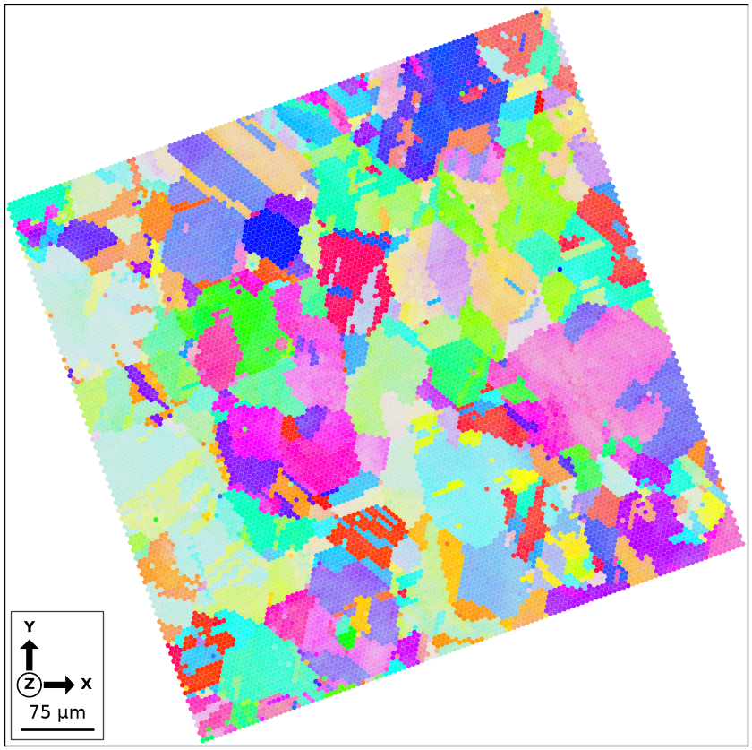
The map is turned on screen, while the object summary still identifies a hexagonal grid. If the same data arrives as a plain list, gridify recovers the rotated lattice without requiring axis alignment.

gridify(ebsdR.flatten())

EBSD (y↑→x)
  size: 136 × 119 grid
  Phase  Orientations  Mineral  Color         Symmetry  Crystal reference frame
  1      16116 (100%)  Copper   LightSkyBlue  m-3m      Copper
  properties : confidenceindex, extra1, extra2, extra3, extra4, fit, grainId, imagequality, semsignal
  scan unit  : um
  X × Y      : [-198.5 → 554.4] × [0 → 750.3]
  hex lattice: spacing 5

Robustness to Distorted Grids

EBSD is measured on a tilted specimen. Seen from a finite working distance, the far edge is farther away and appears smaller. The measured positions can therefore depart smoothly from any single rigid lattice. MTEX still reconstructs the underlying grid indices of an EBSD object. This matters to gridify and to every operation that needs neighbours, including calcGrains and the cell drawing of a map.

Grid reconstruction uses a local deformation model. MTEX first fits an ideal affine grid. It then interpolates the local deviation between the measured positions and that grid wherever a cell has no measurement. Thus a gap, a notIndexed hole, and the dummy cells used to bound the map follow the measured distortion rather than an unrelated rigid lattice.

These terms are distinct. A gap is a run of measurements removed from a scan line, such as by selecting one phase. A hole is a connected notIndexed area inside the scanned region. A dummy cell is a synthetic cell beyond the scanned edge; it has no id and never becomes a grain.

The example uses a real map because the failure appears only when the map is realistically wide. A small synthetic grid remains safe at distortion levels that already misindex a wide map.

ebsd = mtexdata('small')

transform moves every pixel and its unit cell. It leaves orientations and all other per-pixel properties untouched. The command takes a spatialTransform, which records the mapping as an object; see Spatial Transforms.

A tilt is a projective transform. Straight lines remain straight, but parallel lines need not, and scale varies across the frame. Three values specify it: the surface tilt, the working distance, and the point left in place. byTilt tilts about the x axis, so the tilt angle foreshortens the map across that axis, along y. The working distance controls perspective, which vanishes as that distance grows.

Here the tilt is known and imposed. Recovering an unknown tilt from two measured images is the inverse problem. spatialTransformTilt fits it in stages.

theta = 20 * degree                                  # surface tilt
wd = 8 * (ebsd.pos.y.max() - ebsd.pos.y.min())       # working distance
centre = mean(ebsd.pos)                              # what the tilt leaves in place

distort = spatialTransformProjective.byTilt(theta, wd, centre)
distort

spatialTransformProjective
  model       stage  parameters
  projective  ·      perspective (0, -1.31e-05)

The map is compressed along y, from 3000 to 2820 micrometres, while the x extent is left alone by the tilt and only stretched by perspective. It tapers towards the edge that is farther away.

ebsdDistorted = transform(ebsd, distort)

plot(ebsdDistorted['Fo'], ebsdDistorted['Fo'].orientations)
hold(True)
plot(ebsdDistorted['En'], ebsdDistorted['En'].orientations)
plot(ebsdDistorted['Di'], ebsdDistorted['Di'].orientations)
hold(False)

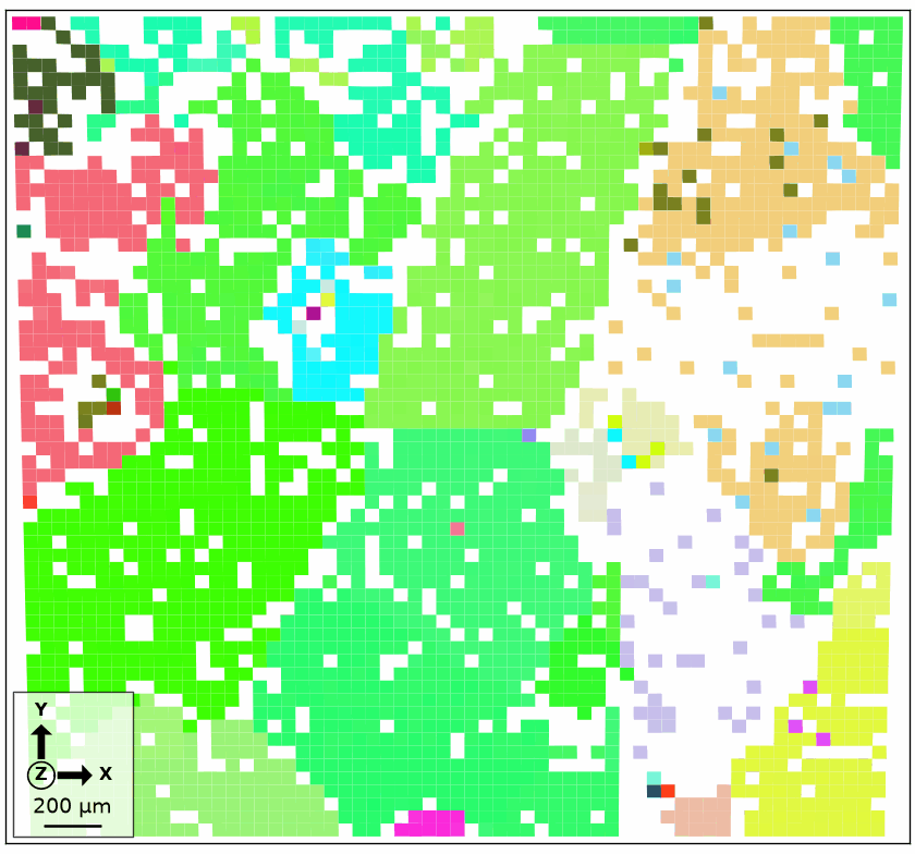
The following pair measures the imposed distortion in cell units. Its first value is the maximum pixel displacement. Its second is the largest residual after the best affine grid has been removed.

pos0 = ebsd.pos.data.reshape(-1, 3)[:, :2]
posD = ebsdDistorted.pos.data.reshape(-1, 3)[:, :2]
ijD = ebsdDistorted.lattice.ij.astype(float)
isIndexed = ebsdDistorted.isIndexed.reshape(-1)
affineDesign = np.column_stack([np.ones(len(ijD)), ijD])
affineFit = np.linalg.lstsq(affineDesign[isIndexed], posD[isIndexed], rcond=None)[0]
cellSize = ebsd.lattice.dxy
distortionInCells = np.array([np.linalg.norm(posD - pos0, axis=1).max(),
                              np.linalg.norm(posD - affineDesign @ affineFit, axis=1).max()]) / cellSize
distortionInCells

array([2.48  , 0.8041])

Every pixel has moved by up to 2.48 cells. Once the affine foreshortening is removed, 0.80 cell remains. That is enough for a rigid reconstruction to round a pixel onto its neighbour’s site. Even so, the same grid indices are recovered as for the undistorted map.

np.array_equal(ebsdDistorted['Fo'].lattice.ij, ebsd['Fo'].lattice.ij)

True

Drawing each measurement as its unit cell shows the result. The cells form one continuous deformed mesh, with no cell sheared independently of its neighbours. A rigid reconstruction would make the mesh wavy and would give calcGrains the wrong neighbours.

plot(ebsdDistorted['Fo'], ebsdDistorted['Fo'].orientations, edgeColor='black')
hold(True)
plot(ebsdDistorted['En'], ebsdDistorted['En'].orientations, edgeColor='black')
plot(ebsdDistorted['Di'], ebsdDistorted['Di'].orientations, edgeColor='black')

# grain reconstruction consequently sees the distorted map as the same neighbourhood graph
grains = calcGrains(ebsdDistorted, minPixel=3)
grains = smoothBoundary(grains, simplify=False)

plot(grains.boundary, lineWidth=2)
hold(False)
grains

grain2d (y↑→x)
  size: 24
  Phase  Grains            Mineral     Color         Symmetry  Crystal reference frame
  1      15 (1943 pixels)  Forsterite  LightSkyBlue  mmm       Forsterite
  2      3 (284 pixels)    Enstatite   DarkSeaGreen  mmm       Enstatite
  3      6 (240 pixels)    Diopside    Goldenrod     12/m1     Diopside
  boundary segments: 1091, inner: 30, triple points: 22

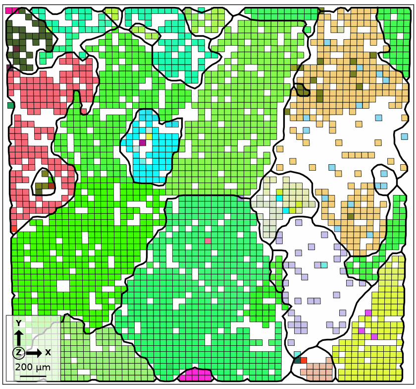
The boundary overlay remains closed and follows the tapered map. No duplicated or missing grain strips appear along its edges.

Gridded EBSD Data