EBSD.smooth

A method of EBSD.

the map with its orientations denoised, every one replaced by one computed from its neighbours, within the grains where the map knows them and within the phases otherwise

Syntax

ebsd_s = smooth(ebsd)

ebsd_s = smooth(ebsd, halfQuadraticFilter())

ebsd_s = smooth(ebsd, F, fill=True)

ebsd_s = smooth(ebsd, F, fill=grains)

ebsd_s = smooth(ebsd, F, props=('bc',))

Description

The orientations are turned into a field of tangent vectors per connected component of the map (a grain, if calcGrains has written the grain ids, else a phase) and the filter acts on that field: a variational filter (splineFilter, halfQuadraticFilter, l1TVFilter, infimalConvolutionFilter) solves for the smoothed field, a window filter (meanFilter, medianFilter, KuwaharaFilter) replaces each pixel by its neighbourhood. Nothing is mixed across a grain boundary or a phase boundary.

With fill the pixels that carry no measurement are solved for too (this is not the same as notIndexed); fill=grains fills a pixel only from the grain whose polygon holds it, so pixels between grains stay empty. A window filter solves for nothing, so with it the holes are closed by fill first. The map passed is not changed; MATLAB’s second output, the filter, is the F passed.

Input

Keywords

Output

Example

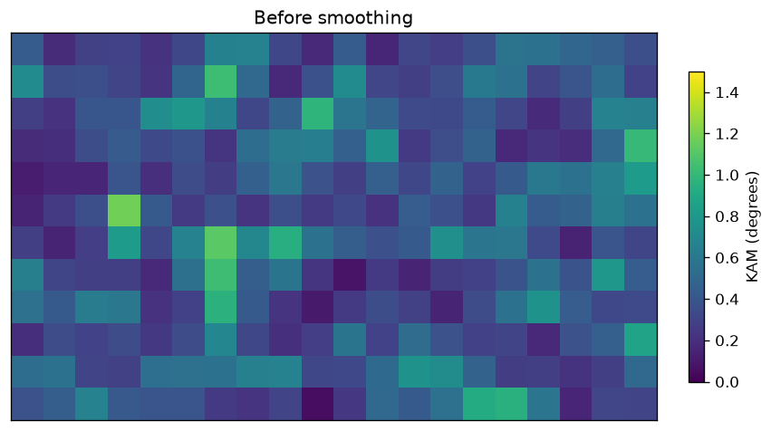
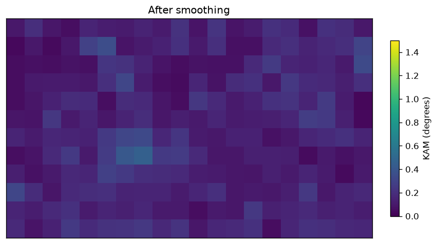
Denoise a synthetic map containing two grains and reproducible orientation noise. Reconstruct the grains first so the filter respects their boundary.

import numpy as np
import matplotlib.pyplot as plt
from mtex import (EBSD, crystalFrame, phaseList, rotation, vector3d, degree,
                  calcGrains, smooth, meanFilter, KAM, plot, mtexColorbar, mtexTitle, newMtexFigure)

x, y = np.meshgrid(np.arange(20), np.arange(12))
base = np.where(x < 10, 0.0, 20.0)
noise = np.random.default_rng(7).normal(0, 0.4, x.shape)
rot = rotation.byAxisAngle(vector3d.Z, (base + noise).ravel()*degree)
cs = crystalFrame('m-3m')
ebsd = EBSD(np.c_[x.ravel(), y.ravel()], rot, np.ones(x.size, dtype=int), phaseList(cs))
grains = calcGrains(ebsd, angle=10*degree)
filtered = smooth(ebsd, meanFilter(numNeighbours=1))
for data, title in ((ebsd, 'Before smoothing'), (filtered, 'After smoothing')):
    newMtexFigure()
    kam = KAM(data)/degree
    print(title, 'median KAM (degrees):', round(float(np.nanmedian(kam)), 3))
    plot(data, kam, colorRange=(0, 1.5), micronbar=False)
    mtexColorbar(title='KAM (degrees)')
    mtexTitle(title)
print('Grain ids unchanged:', np.array_equal(filtered.grainId, ebsd.grainId))
plt.show()

The returned map has new orientations and retains the original segmentation. Lower KAM shows reduced local variation in this synthetic example; it is not a general measure of denoising quality. Choose a filter and length scale appropriate to the features to retain.

Before smoothing median KAM (degrees): 0.373
After smoothing median KAM (degrees): 0.141
Grain ids unchanged: True

See also

fill, interp, halfQuadraticFilter, splineFilter, meanFilter, EBSDDenoising, EBSDFilling

MATLAB’s EBSD.smooth

@article{bachmann2010mtex,
  author  = {F. Bachmann and R. Hielscher and H. Schaeben},
  title   = {Texture Analysis with MTEX - Free and Open Source Software Toolbox},
  journal = {Solid State Phenomena},
  volume  = {160},
  pages   = {63-68},
  year    = {2010},
  doi     = {10.4028/www.scientific.net/SSP.160.63},
  url     = {https://doi.org/10.4028/www.scientific.net/SSP.160.63}
}