Denoising Orientation Maps

Every measured orientation has uncertainty. Some errors are systematic: an incorrect pattern centre or reference frame can bias a whole map in a related way. A filter cannot discover that bias from the map alone. Check the setup as described in Reference Frames before treating point-to-point variation as noise.

Random errors appear instead as scatter between nearby measurements. This page reduces that scatter while trying to preserve real orientation gradients and abrupt changes inside grains. Filling measurements whose phase is notIndexed is a different operation; see Filling Missing Data.

The examples assume that you can reconstruct grains and read an orientation map. Those steps are introduced in Grain Reconstruction and IPF Maps. A quantitative comparison of the filters and their effect on KAM and GND calculations is given by Hielscher et al. (2019).

import numpy as np

from mtex import *

Making the noise visible

The example is a map of deformed magnesium. Its plotting convention is set explicitly so that the specimen frame does not depend on the current MTEX session.

# import the data
plottingConvention.default('y↑→x')
ebsd = mtexdata('twins')

# reconstruct the grain structure
grains = calcGrains(ebsd, angle=10 * degree, minPixel=5)

# smooth grain boundaries
grains = smoothBoundary(grains, 5)

# consider only indexed data
ebsd = ebsd['indexed']

# plot the orientation map
ipfKey = ipfColorKey(ebsd.CS.properGroup())
plot(ebsd, ipfKey.orientation2color(ebsd.orientations))

# and on top the grain boundaries
hold(True)
plot(grains.boundary, lineWidth=2, lineColor='white')
hold(False)

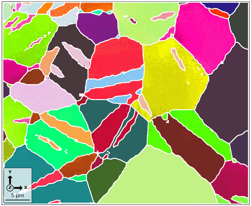
The grains appear almost uniformly coloured. This does not show that the measurements are noise-free: the IPF key displays absolute orientation, and sub-degree differences produce only small colour changes.

A more sensitive view compares every orientation with the original mean orientation of its grain. Hue represents the misorientation axis and saturation represents its angle. This colour scheme follows Thomsen et al. (2017).

# use the original grain means as reference orientations
grainMean = grains.selectByGrainId(ebsd.grainId).meanOrientation
colorKey = axisAngleColorKey(ebsd)
colorKey.oriRef = grainMean

# keep one colour scale for every comparison on this page
rawDeviation = angle(ebsd.orientations, grainMean)
colorKey.maxAngle = np.nanquantile(rawDeviation, 0.8)

plot(ebsd, colorKey.orientation2color(ebsd.orientations))
hold(True)
plot(grains.boundary, lineWidth=2)
hold(False)

print(f'Raw mean deviation from the grain mean: {np.nanmean(rawDeviation) / degree:.2f} degree')

Raw mean deviation from the grain mean: 0.70 degree

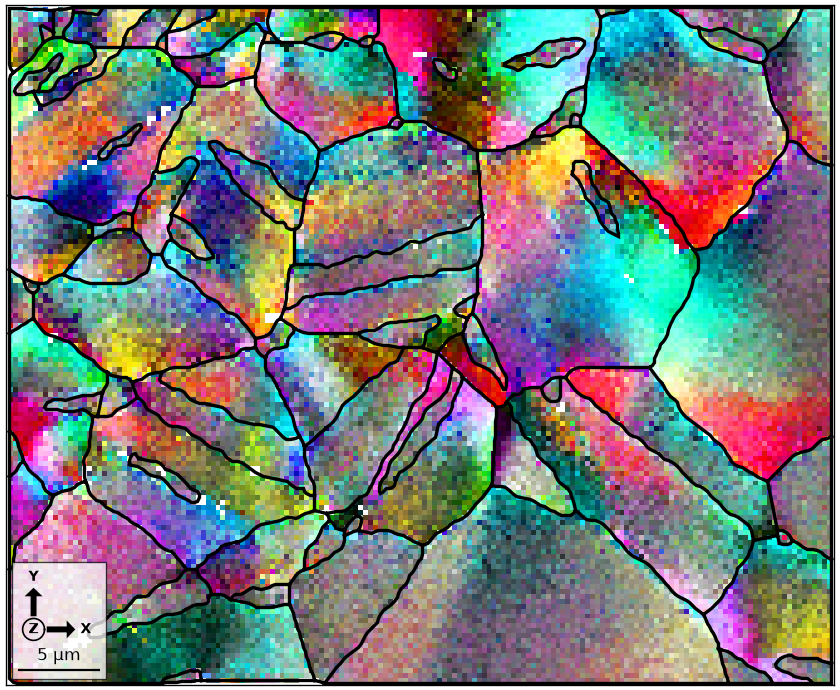
Two patterns now separate. Smooth colour gradients across the larger grains record lattice bending in the deformed crystal. Pixel-to-pixel speckle superposed on those gradients is the signature to reduce. The printed mean contains both effects, so its decrease is a diagnostic of smoothing rather than a direct measurement of the noise amplitude.

How smooth uses the grain structure

Every filter on this page is applied with smooth. Because calcGrains assigned ebsd.grainId, smooth treats each grain separately. It therefore does not average orientations across a reconstructed grain boundary. An abrupt change inside one reconstructed grain is a subgrain boundary, and whether it survives depends on the filter.

Denoising changes the orientations in the returned map. It does not reconstruct the grains or move their boundaries, which is why the same original boundaries are overlaid throughout. Reconstruct the grains again only if the denoised orientations should define a new segmentation.

Two variational filters are useful in practice. The total variation filter favours sharp internal changes; the smoothing spline favours a continuously curved map.

The total variation filter

The halfQuadraticFilter balances fidelity to the measured orientations against first-order smoothness over the map. Its default total variation model permits jumps, so it can preserve a subgrain boundary instead of averaging across it. This method for rotation-valued images is described by Bergmann et al. (2016) and builds on the total variation model of Rudin et al. (1992).

The property F.alpha controls the trade-off; larger values smooth more. The property F.threshold prevents smoothing across neighbour differences above its value. The default settings are used here. Their price is a tendency towards cartoon-like patches and staircases.

F = halfQuadraticFilter()

# smooth the data
ebsdS = smooth(ebsd, F)
ebsdS = ebsdS['indexed']

# plot the smoothed data on the fixed colour scale
colorKey.oriRef = grains.selectByGrainId(ebsdS.grainId).meanOrientation
plot(ebsdS, colorKey.orientation2color(ebsdS.orientations))

hold(True)
plot(grains.boundary, lineWidth=2)
hold(False)

hqDeviation = angle(ebsdS.orientations, colorKey.oriRef)
print(f'Total variation mean deviation: {np.nanmean(hqDeviation) / degree:.2f} degree')

Total variation mean deviation: 0.63 degree

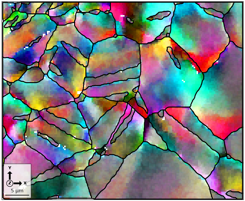
The isolated colour changes are largely gone, while extended gradients and sharp internal changes remain. Read the printed reduction together with the map: the remaining deviation includes real deformation and should not be driven to zero.

The smoothing spline filter

The splineFilter is the filter that smooth uses when none is supplied. It penalizes curvature rather than first-order variation. The result is rounder than the total variation result, but fine subgrain boundaries are smoothed with the noise.

In MATLAB it is the only filter on this page that selects its own regularization parameter, by generalized cross-validation with robust smoothing by default, following Garcia (2010); that automatic mode is not fully supported on hexagonal grids there. Here every variational filter takes a smoothing length, four lattice steps by default, and the spline is applied with that length.

F = splineFilter()

# smooth the data
ebsdS = smooth(ebsd, F)
ebsdS = ebsdS['indexed']

# plot the smoothed data on the fixed colour scale
colorKey.oriRef = grains.selectByGrainId(ebsdS.grainId).meanOrientation
plot(ebsdS, colorKey.orientation2color(ebsdS.orientations))

hold(True)
plot(grains.boundary, lineWidth=2)
hold(False)

splineDeviation = angle(ebsdS.orientations, colorKey.oriRef)
print(f'Spline mean deviation: {np.nanmean(splineDeviation) / degree:.2f} degree')

Spline mean deviation: 0.64 degree

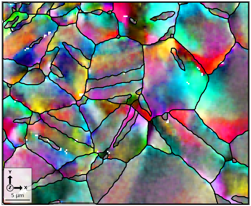
The printed mean deviation is close to the total variation result, but the spatial result is not the same: the spline makes the colour fields rounder and removes more of the fine internal structure.

Technical details - further filters

The filters below are retained for comparison and completeness. In practice they are inferior to the two above for this map. The first three are sliding-window filters: each orientation is replaced by a value computed only from a local neighbourhood.

The mean filter

The meanFilter replaces each orientation by a local mean. A radius of one gives the smallest neighbourhood.

F = meanFilter()
F.numNeighbours = 1

# smooth the data
ebsdS = smooth(ebsd, F)
ebsdS = ebsdS['indexed']

# plot the smoothed data on the fixed colour scale
colorKey.oriRef = grains.selectByGrainId(ebsdS.grainId).meanOrientation
plot(ebsdS, colorKey.orientation2color(ebsdS.orientations))

hold(True)
plot(grains.boundary, lineWidth=2)
hold(False)

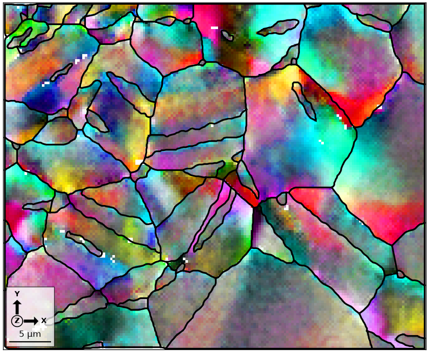
The isolated speckle is weaker, but the extended colour fields have also spread. A local mean has no criterion for distinguishing a noisy jump from a real one inside the grain.

Increasing F.numNeighbours broadens the spatial support. More noise is removed, at the cost of blurring every internal feature further.

F.numNeighbours = 3

# smooth the data
ebsdS = smooth(ebsd, F)
ebsdS = ebsdS['indexed']

# plot the smoothed data on the fixed colour scale
colorKey.oriRef = grains.selectByGrainId(ebsdS.grainId).meanOrientation
plot(ebsdS, colorKey.orientation2color(ebsdS.orientations))

hold(True)
plot(grains.boundary, lineWidth=2)
hold(False)

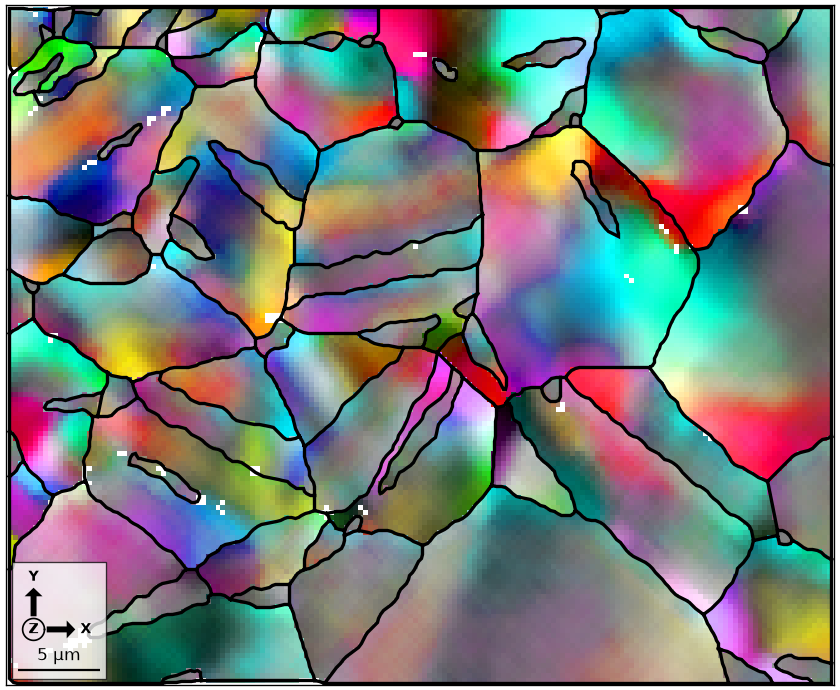
Compared with the preceding map, the broader patches and weaker narrow features show the cost of increasing the neighbourhood.

The median filter

A mean is pulled towards one bad measurement and averages across every internal step. The medianFilter selects the neighbouring orientation with the smallest mean distance to the others. It is therefore more robust to isolated outliers and more likely to preserve a subgrain boundary.

F = medianFilter()

# use a 7-by-7 window
F.numNeighbours = 3

# smooth the data
ebsdS = smooth(ebsd, F)
ebsdS = ebsdS['indexed']

# plot the smoothed data on the fixed colour scale
colorKey.oriRef = grains.selectByGrainId(ebsdS.grainId).meanOrientation
plot(ebsdS, colorKey.orientation2color(ebsdS.orientations))

hold(True)
plot(grains.boundary, lineWidth=2)
hold(False)

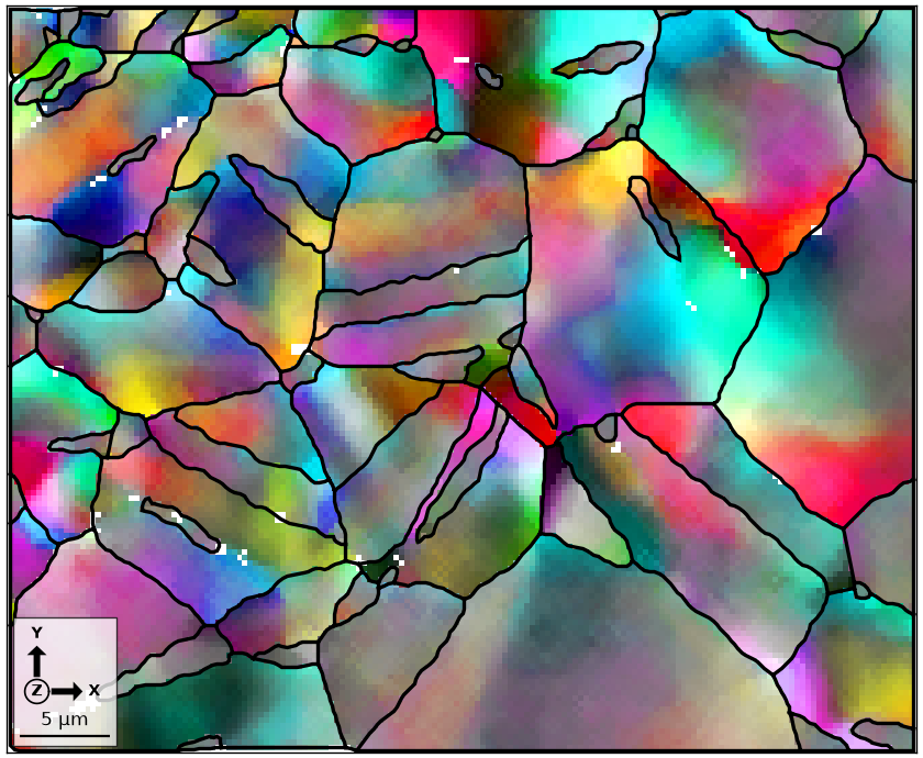
The map breaks into cartoon-like patches with visible steps. This staircase effect is what the median does to a gentle orientation gradient.

The Kuwahara filter

The KuwaharaFilter is also designed to survive outliers and preserve subgrain boundaries. It divides the neighbourhood into four overlapping quadrants and uses the mean of the most uniform one. The block structure in the result shows why it is rarely satisfactory in practice.

F = KuwaharaFilter()
F.numNeighbours = 5

# smooth the data
ebsdS = smooth(ebsd, F)
ebsdS = ebsdS['indexed']

# plot the smoothed data on the fixed colour scale
colorKey.oriRef = grains.selectByGrainId(ebsdS.grainId).meanOrientation
plot(ebsdS, colorKey.orientation2color(ebsdS.orientations))

hold(True)
plot(grains.boundary, lineWidth=2)
hold(False)

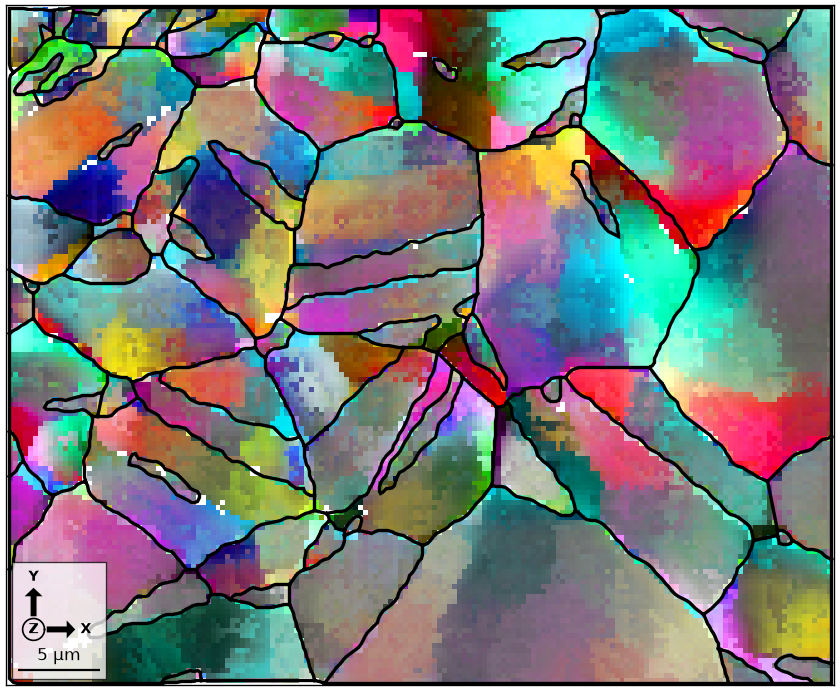
Large rectangular colour patches follow the selected subwindows rather than the smooth gradients visible in the raw map.

The infimal convolution filter

The infimalConvolutionFilter combines first- and second-order penalties. A linear gradient can then survive where plain total variation tends to create a staircase, while a sharp internal boundary can remain. The model is described by Bergmann et al. (2017). This implementation is still under development and is not recommended for routine use. Its two weights, alpha for the first-order and beta for the second-order penalty, are derived from the smoothing length; MATLAB names them lambda and mu.

F = infimalConvolutionFilter()

# smooth the data
ebsdS = smooth(ebsd, F)
ebsdS = ebsdS['indexed']

# plot the smoothed data on the fixed colour scale
colorKey.oriRef = grains.selectByGrainId(ebsdS.grainId).meanOrientation
plot(ebsdS, colorKey.orientation2color(ebsdS.orientations))

hold(True)
plot(grains.boundary, lineWidth=2)
hold(False)

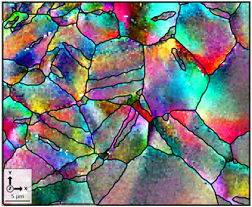
The result is smoother within gradients than the total variation map and sharper at internal steps than the spline map. It offers no practical advantage here that outweighs its experimental status.

Choosing a filter

Use the halfQuadraticFilter when preserving subgrain boundaries matters. Use the splineFilter on a square grid when smooth gradients matter more. In either case, vary the smoothing strength and check that persistent spatial features remain; a lower mean deviation alone does not prove that the result is better.

Denoising is usually preparation for a noise-sensitive calculation. Kernel Average Misorientation and Grain Reference Orientation Deviation continue with the same distinction between point-to-point scatter and real lattice bending.

@article{bachmann2010mtex,
  author  = {F. Bachmann and R. Hielscher and H. Schaeben},
  title   = {Texture Analysis with MTEX - Free and Open Source Software Toolbox},
  journal = {Solid State Phenomena},
  volume  = {160},
  pages   = {63-68},
  year    = {2010},
  doi     = {10.4028/www.scientific.net/SSP.160.63},
  url     = {https://doi.org/10.4028/www.scientific.net/SSP.160.63}
}