Kernel Average Misorientation (KAM)

This page is not yet compared with the MATLAB page.

The kernel average misorientation asks a local question: by how much does the orientation at one measurement differ from the orientations at nearby measurements? Averaging those disorientation angles gives one non-negative angle per pixel. A KAM map therefore highlights abrupt local orientation changes and gradual lattice bending.

KAM is sensitive to dislocation structures, but it is not a direct map of dislocations or plastic strain. It keeps only the disorientation angle, not the axis, and a two-dimensional map contains only part of the lattice curvature. The scan step size, neighbourhood, angular precision, grain segmentation, and any preprocessing all affect the value.

This page assumes familiarity with grain reconstruction and misorientations. Unlike the grain reference orientation deviation in Mis2Mean / GROD, KAM compares a measurement only with nearby measurements. It says how sharply the orientation changes locally, not how far the grain as a whole has turned.

import numpy as np

from mtex import *
from mtex.maps.phaselist import PHASE_COLOR_ORDER

A deformed ferrite specimen

The example uses a deformed ferrite map. Its plotting convention is set explicitly so that the map does not inherit one from the current MTEX session.

plottingConvention.default('y↓→x')
ebsd = mtexdata('ferrite')

# reconstruct grains and store one grain id per measurement
grains = calcGrains(ebsd, minPixel=8)

# smooth the outlines used as overlays
grains = smoothBoundary(grains, 5)

# plot the indexed orientations and reconstructed grain boundaries
ebsdIndexed = ebsd['indexed']
ipfKey = ipfColorKey(ebsdIndexed.CS)
ipfColor = ipfKey.orientation2color(ebsdIndexed.orientations)
plot(ebsdIndexed, ipfColor)
hold(True)
plot(grains.boundary, lineWidth=1.5)
hold(False)

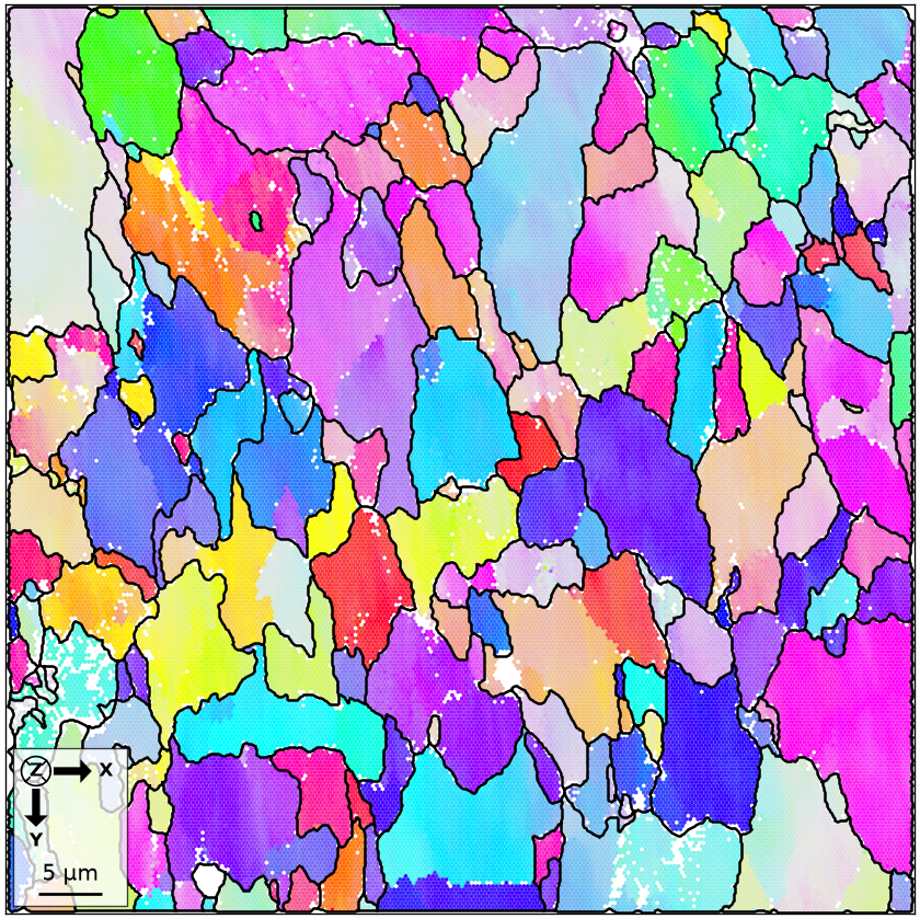
The colours show the orientation field, while the black lines mark the reconstructed grain boundaries. The following KAM calculations use those boundaries as barriers, but smoothing the drawn outlines does not change which measurement belongs to which grain.

The nearest-neighbour KAM

ebsd.KAM returns an angle in radians. Dividing by degree converts it to degrees. The default uses first-order neighbours, applies no angular threshold, and excludes pairs in different grains when ebsd.grainId is present.

kamRaw = ebsd.KAM() / degree

print(f'Default KAM median: {np.nanmedian(kamRaw):.2f} degree; maximum: {np.nanmax(kamRaw):.1f} degree')

plot(ebsd, kamRaw, micronbar=False)
setColorRange([0, 15])
mtexColorMap('LaboTeX')
mtexColorbar(title='KAM in degree')
hold(True)
plot(grains.boundary, lineWidth=1.5)
hold(False)

Default KAM median: 0.60 degree; maximum: 24.6 degree

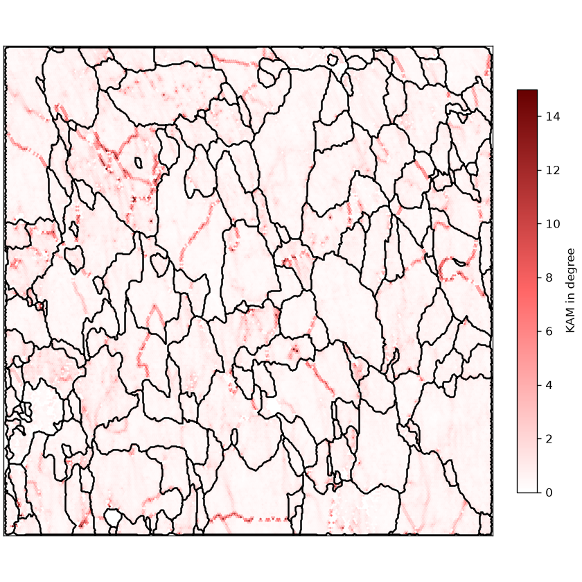
The median is 0.60°. The colour range makes the network of large values inside the grains stand out as red lines. These are abrupt internal orientation changes associated with subgrain boundaries and other local dislocation structures. They are more than an order of magnitude above the background, so the weaker variation receives little colour contrast.

Measurements whose phase is notIndexed have no usable orientation and therefore no KAM. MTEX also excludes a neighbour in a different phase.

Applying an angular threshold

The option threshold rejects an individual neighbour pair when its disorientation angle is larger than \(\delta\). It does not classify or remove a boundary. A 2.5° threshold therefore suppresses only the contributions above 2.5°; a lower-angle subgrain boundary can remain in the map.

kamThreshold = ebsd.KAM(threshold=2.5 * degree) / degree

print(f'Thresholded KAM median: {np.nanmedian(kamThreshold):.2f} degree')

plot(ebsd, kamThreshold, micronbar=False)
setColorRange([0, 2])
mtexColorMap('LaboTeX')
mtexColorbar(title='KAM in degree')
hold(True)
plot(grains.boundary, lineWidth=1.5)
hold(False)

Thresholded KAM median: 0.59 degree

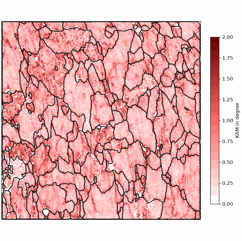
Most of the red network has gone, and the smaller colour range reveals gentle bending between the strongest internal boundaries. The map is also visibly speckled. The remaining differences are a few tenths of a degree, which is comparable with the orientation uncertainty of conventional Hough-indexed EBSD data.

Rejecting a pair also removes it from the denominator of the average. Pixels near boundaries and holes may therefore be averaged over fewer neighbours. If no eligible neighbour remains, the result is NaN.

Increasing the neighbourhood

One way to reduce speckle is to include all neighbours up to three nearest-neighbour steps away.

kamOrder3 = ebsd.KAM(threshold=2.5 * degree, order=3) / degree

print(f'Third-order thresholded KAM median: {np.nanmedian(kamOrder3):.2f} degree')

plot(ebsd, kamOrder3, micronbar=False)
setColorRange([0, 2])
mtexColorMap('LaboTeX')
mtexColorbar(title='KAM in degree')
hold(True)
plot(grains.boundary, lineWidth=1.5)
hold(False)

Third-order thresholded KAM median: 0.81 degree

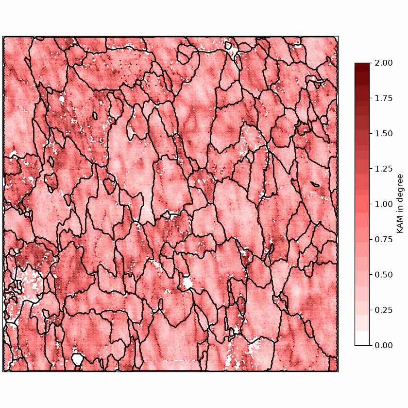
The result is smoother, but order=3 is not merely stronger averaging. It measures orientation differences over a larger physical distance. The median rises from 0.59° to 0.81° because more distant measurements have accumulated more orientation change. Fine structures are broadened along with the noise.

For maps with different step sizes, the same order does not represent the same distance. The option radius can instead select neighbours by physical distance, and weights can weight them by that distance. KAM remains an angle average, however, not an orientation gradient normalized by distance. The flag max=True returns the largest eligible neighbour angle instead of the average.

Denoising before computing KAM

A second approach keeps the first-order neighbourhood and reduces random scatter in the orientations before computing KAM. See Denoising for the filter assumptions and alternatives.

# choose a total variation filter
F = halfQuadraticFilter()
F.alpha = 0.5

# denoise within the reconstructed grains and fill missing lattice sites
ebsdS = smooth(ebsd, F, fill=True)

# compute the first-order KAM from the denoised orientations
kamDenoised = ebsdS.KAM(threshold=2.5 * degree) / degree

print(f'Denoised first-order KAM median: {np.nanmedian(kamDenoised):.2f} degree')

plot(ebsdS, kamDenoised, micronbar=False)
setColorRange([0, 2])
mtexColorMap('LaboTeX')
mtexColorbar(title='KAM in degree')
hold(True)
plot(grains.boundary, lineWidth=1.5)
hold(False)

Denoised first-order KAM median: 0.20 degree

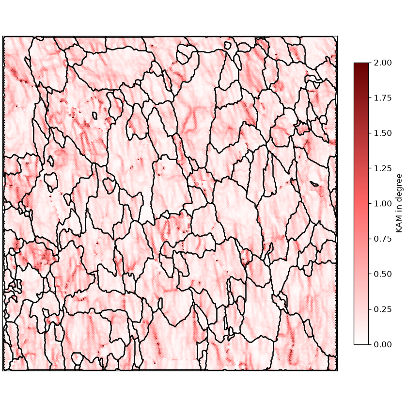
For this example, this is the map to use when examining weak continuous structure. Its median is well below half the 0.59° obtained with thresholding alone. The surviving features run continuously through the grains rather than appearing as isolated pixels, which is consistent with local deformation structures.

The numerical drop does not prove that more than half of the original KAM was measurement error. Denoising changes noise and real signal together, and its parameters affect both. Compare KAM values quantitatively only when acquisition step size, neighbourhood, threshold, segmentation, and preprocessing are controlled.

The definition

Write \(o_{i,j}\) for the orientation at pixel \((i,j)\) and \(N(i,j)\) for the eligible neighbours counted there. For the unweighted mean,

Here \(\omega\) is the disorientation angle between two orientations, and \(\lvert N(i,j)\rvert\) is the number of eligible neighbours. MTEX constructs \(N(i,j)\) from the following choices:

• neighbours up to order \(n\), meaning \(n\) steps on the scan grid
• or neighbours within a physical radius
• only indexed neighbours belonging to the same phase
• only neighbours in the same reconstructed grain when grainId exists
• only neighbours at or below the threshold angle \(\delta\)

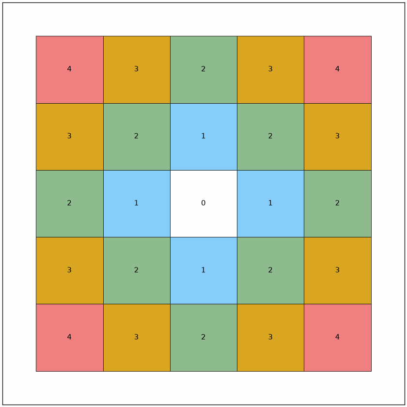
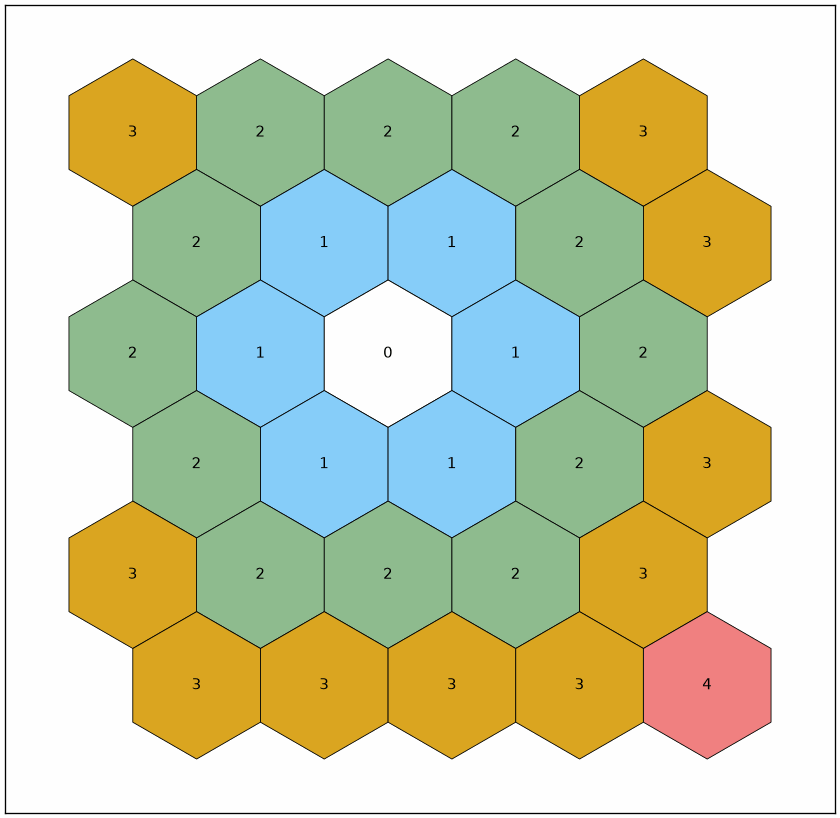
Denoising changes the orientations \(o_{i,j}\) before this calculation; it does not change the definition of \(N(i,j)\). The diagrams number the graph distance from the centre pixel. Notice that the square grid grows as a diamond of four-neighbour steps, while the hexagonal grid grows in six-sided rings.

# the neighbourhood diagrams: a map of five phases coloured by the graph distance
def ringMap(N, hexagonal=False):
  i, j = np.indices(N.shape)
  csList = [crystalFrame('1', mineral=f'{k} steps', color=PHASE_COLOR_ORDER[k]) for k in range(5)]
  if hexagonal:
    x, y = 10.0 * (j + 0.5 * (i % 2)), 10.0 * np.sqrt(3) / 2 * i
    a = np.arange(6) * np.pi / 3 + np.pi / 6
    cell = vector3d(10 / np.sqrt(3) * np.cos(a), 10 / np.sqrt(3) * np.sin(a), 0)
  else:
    x, y, cell = 10.0 * j, 10.0 * i, None
  pos = np.column_stack([x.ravel(), y.ravel(), np.zeros(N.size)])
  return EBSD(pos, rotation(np.full((N.size, 4), np.nan)), N.ravel(), csList, unitCell=cell)

square = ringMap(np.array([[4, 3, 2, 3, 4], [3, 2, 1, 2, 3], [2, 1, 0, 1, 2], [3, 2, 1, 2, 3], [4, 3, 2, 3, 4]]))
hexagonal = ringMap(np.array([[3, 2, 2, 2, 3], [2, 1, 1, 2, 3], [2, 1, 0, 1, 2], [2, 1, 1, 2, 3], [3, 2, 2, 2, 3], [3, 3, 3, 3, 4]]), hexagonal=True)

plot(square, edgeColor='black', micronbar=False, backend='patch', legend=False)
text(square, square.phaseId.ravel())
plot(hexagonal, edgeColor='black', micronbar=False, backend='patch', legend=False)
text(hexagonal, hexagonal.phaseId.ravel())

References

• M. Kamaya, Assessment of Local Deformation Using EBSD: Quantification of Accuracy of Measurement and Definition of Local Gradient, Ultramicroscopy 111 (2011), 1189–1199. This paper explains why local misorientation depends on measurement accuracy and the distance between measurements.
• R. R. Shen and P. Efsing, Overcoming the Drawbacks of Plastic Strain Estimation Based on KAM, Ultramicroscopy 184 (2018), 156–163. It treats the effects of noise, kernel, step size, and grain size on quantitative comparisons.
• R. Hielscher, C. B. Silbermann, E. Schmidl, and J. Ihlemann, Denoising of Crystal Orientation Maps, Journal of Applied Crystallography 52 (2019), 984–996. It compares orientation filters and their effects on KAM and curvature estimates.
• A. J. Schwartz, M. Kumar, B. L. Adams, and D. P. Field, editors, Electron Backscatter Diffraction in Materials Science, 2nd ed., Springer, 2009. This is a broad reference for EBSD measurement, uncertainty, and deformation analysis.

@article{bachmann2010mtex,
  author  = {F. Bachmann and R. Hielscher and H. Schaeben},
  title   = {Texture Analysis with MTEX - Free and Open Source Software Toolbox},
  journal = {Solid State Phenomena},
  volume  = {160},
  pages   = {63-68},
  year    = {2010},
  doi     = {10.4028/www.scientific.net/SSP.160.63},
  url     = {https://doi.org/10.4028/www.scientific.net/SSP.160.63}
}