Grain Reconstruction

A grain is a phase-homogeneous, spatially connected region of EBSD pixels produced by segmentation. A phase change between neighbouring pixels is always a grain boundary. Within one phase, the usual segmentation rule asks whether the orientations differ by more than a chosen angle. The command that applies these rules is calcGrains.

This page assumes that you can select and plot an EBSD map. If the angle between two orientations is new to you, first see Misorientation Theory.

Three settings shape the result. They are the boundary misorientation angle, the treatment of measurements that could not be indexed, and the minimum number of pixels returned as a grain. They are segmentation choices, not properties measured independently from the specimen. We take them one at a time on a map that exercises all three.

import matplotlib.pyplot as plt
import numpy as np

from mtex import *

# import the data
plottingConvention.default('y↑→x')
ebsd = mtexdata('forsterite')

# restrict it to a subregion of interest
ebsd = ebsd[ebsd.inpolygon(np.array([5, 2, 10, 5]) * 1e3)]
ebsd

EBSD (y↑→x)
  size: 20301
  Phase  Orientations  Mineral     Color         Symmetry  Crystal reference frame
  0      4052 (20%)    notIndexed
  1      14093 (69%)   Forsterite  LightSkyBlue  mmm       Forsterite
  2      1397 (6.9%)   Enstatite   DarkSeaGreen  mmm       Enstatite
  3      759 (3.7%)    Diopside    Goldenrod     12/m1     Diopside
  properties    : bands, bc, bs, error, mad
  scan unit     : um
  X × Y         : [5000 → 1.5e+04] × [2000 → 7000]
  square lattice: spacing 50

# make a phase plot
plot(ebsd, micronbar=False)

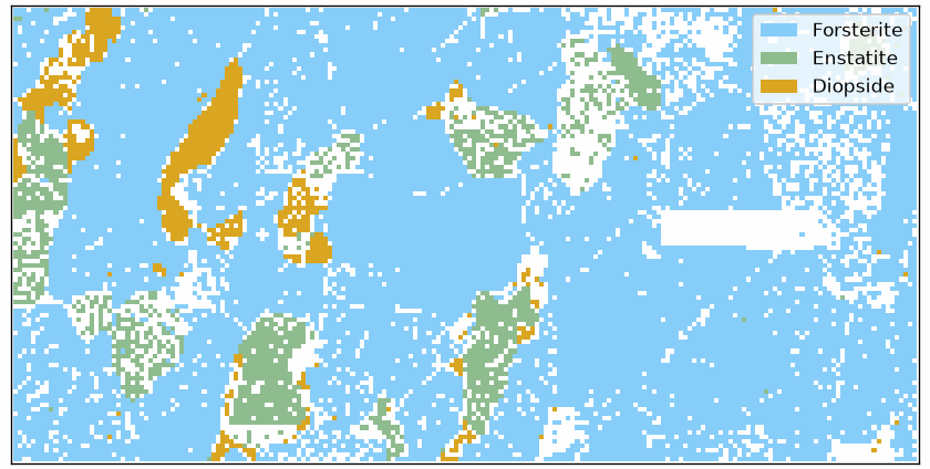
The colours are the phases: forsterite, enstatite and diopside. The white speckle is the first phase in the displayed summary, notIndexed. Its diffraction patterns could not be indexed. One measurement in five on this map is notIndexed. Most lie where boundaries will be reconstructed.

A first reconstruction

We choose a 10 degree threshold and leave alpha and minPixel at their defaults. The displayed grain2d summary is useful here: it reports the number of grains and their phases.

grains = calcGrains(ebsd, angle=10 * degree)
grains

grain2d (y↑→x)
  size: 211
  Phase  Grains              Mineral     Color         Symmetry  Crystal reference frame
  0      1 (259 pixels)      notIndexed
  1      107 (14093 pixels)  Forsterite  LightSkyBlue  mmm       Forsterite
  2      32 (1397 pixels)    Enstatite   DarkSeaGreen  mmm       Enstatite
  3      71 (759 pixels)     Diopside    Goldenrod     12/m1     Diopside
  boundary segments: 4075, inner: 1, triple points: 248

Each grain is one entry of the list, with its own phase, mean orientation, size and shape. The boundaries are stored separately in grains.boundary, which we plot on top of the map.

plot(ebsd, micronbar=False)
hold(True)
plot(grains.boundary, lineWidth=1.5)
hold(False)

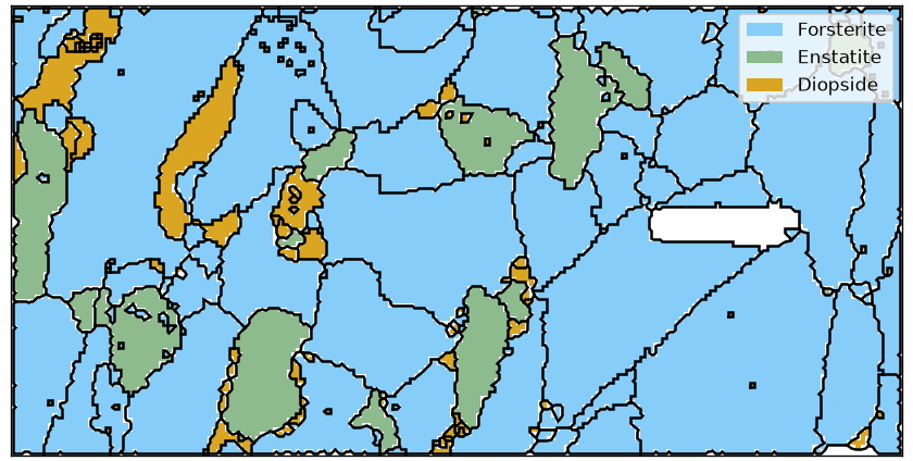
MTEX first partitions the measured surface into one spatial cell per measurement. Neighbouring cells are then connected or separated by the segmentation rule, and connected cells are collected into grains. On this regular grid, the cell edges lie between measurement points. The plotted boundaries therefore follow the grid in steps rather than passing through the points.

Although a fifth of the map is notIndexed, only one grain is notIndexed: the long white bar right of centre. The other notIndexed pixels have been absorbed by adjacent grains. The section on alpha below explains this default behaviour.

The threshold angle

The option angle sets the misorientation above which two neighbouring measurements of the same phase are separated by a boundary. Its default is 15 degrees. Values between 10 and 15 degrees are long-standing conventions, not measurements; see the discussion in the chapter opener.

On a recrystallised map like this one the exact value hardly matters.

for threshold in np.array([2, 5, 10, 15]) * degree:
  g = calcGrains(ebsd, angle=threshold)
  print(f'{round(threshold / degree):2d} degree threshold: {len(g["indexed"]):3d} indexed grains')

 2 degree threshold: 256 indexed grains
 5 degree threshold: 227 indexed grains
10 degree threshold: 210 indexed grains
15 degree threshold: 208 indexed grains

Between 5 and 15 degrees the printed count changes by less than one tenth. It rises sharply only at 2 degrees. Neighbouring measurements on this map are usually either far below all these thresholds or far above them. Few ambiguous pairs lie in between. This is a property of the material, not of the algorithm. It stops being true in the deformed example later on.

Measurements that were not indexed

A notIndexed measurement is not missing from the map. Its diffraction pattern could not be indexed, and MTEX records that fact as the degenerate phase notIndexed. Like any other phase, a connected notIndexed area can form a grain with a boundary around it.

Whether this is what you want depends on the patch. A wide unindexed region is part of the specimen about which you know nothing. It should remain a grain of its own. A one-pixel-wide seam along a grain boundary instead records indexing failure where two lattices overlap. Leaving such a seam creates a spurious grain between the indexed grains on either side.

The option alpha controls the spatial closing that distinguishes these cases. Its value is a radius in multiples of the pixel spacing. A notIndexed area narrower than about 2*alpha pixel spacings is absorbed by the surrounding grains, while a wider area survives. The default is alpha = 3.1.

for alpha in [0, 1, 3.1, 6]:
  g = calcGrains(ebsd, angle=10 * degree, alpha=alpha)
  print(f'alpha = {alpha:3.1f}: {len(g):4d} grains, {len(g["notIndexed"]):4d} of them notIndexed')

alpha = 0.0: 1589 grains, 1064 of them notIndexed
alpha = 1.0:  317 grains,   52 of them notIndexed
alpha = 3.1:  211 grains,    1 of them notIndexed
alpha = 6.0:  209 grains,    0 of them notIndexed

With alpha = 0 nothing is absorbed. The notIndexed pixels then contribute more than one thousand grains of their own, five times the number of indexed grains found with the default. Their seams also divide regions that should be single indexed grains, so the indexed count rises from 210 to 525. A closing radius of one pixel removes almost all of them. The default keeps only the wide notIndexed region, while alpha = 6 absorbs that one too.

The effect is easiest to see when the two extremes are drawn on the same part of the map.

region = np.array([5, 2, 2, 1.5]) * 1e3
ebsdSub = ebsd[ebsd.inpolygon(region)]

grainsSharp = calcGrains(ebsd, angle=10 * degree, alpha=0)

newMtexFigure(layout=[1, 2])

plot(ebsdSub, micronbar=False)
hold(True)
plot(grainsSharp.boundary, lineWidth=1.5)
hold(False)
plt.xlim(region[0], region[0] + region[2]), plt.ylim(region[1], region[1] + region[3])

nextAxis()
plot(ebsdSub, micronbar=False)
hold(True)
plot(grains.boundary, lineWidth=1.5)
hold(False)
plt.xlim(region[0], region[0] + region[2]), plt.ylim(region[1], region[1] + region[3])

((5000.0, 7000.0), (2000.0, 3500.0))

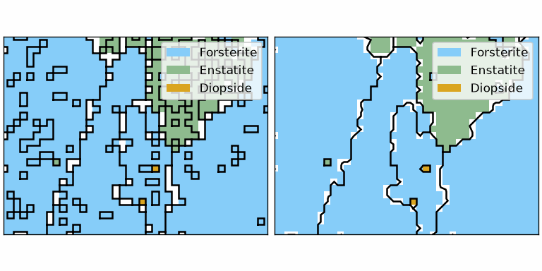
On the left, at alpha = 0, isolated white pixels are fenced off and white seams cut the blue forsterite into pieces. On the right, at the default, the same white measurements remain visible and remain notIndexed, but they no longer separate the surrounding grains. The isolated orange pixels keep boundaries on both sides because they are indexed diopside. The minPixel option below deals with such small indexed grains.

Small indexed grains

Even with the unindexed seams absorbed, a threshold criterion produces grains of one, two or three pixels where a few measurements are mis-indexed. On this map the isolated indexed islands are implausible, but a small grain can be real in another specimen. Inspect the map before choosing a cutoff. The option minPixel removes an indexed grain below the cutoff from the returned list. It marks that grain’s measurements notIndexed rather than merging them into a neighbour. Since it marks them in the map it was given, every step of the sweep below works on a copy of the map.

for minPixel in [1, 5, 10]:
  g = calcGrains(ebsd.copy(), angle=10 * degree, minPixel=minPixel)
  print(f'minPixel = {minPixel:2d}: {len(g["indexed"]):3d} indexed grains, '
        f'holding {100 * np.sum(g["indexed"].numPixel) / np.count_nonzero(ebsd.isIndexed):4.1f}% of the indexed pixels')

minPixel =  1: 210 indexed grains, holding 100.0% of the indexed pixels
minPixel =  5:  90 indexed grains, holding 99.0% of the indexed pixels
minPixel = 10:  71 indexed grains, holding 98.2% of the indexed pixels

More than half of the indexed grains contain fewer than five pixels. Yet together they hold only about one indexed measurement in one hundred. Removing them changes count-based grain statistics greatly. It scarcely changes the large-scale microstructure visible in the map. For a quantitative study, report the cutoff and test nearby values.

Smoothing the boundaries

Because the boundaries run between measurement points, they follow the measurement grid in steps - the staircase effect. This is a property of the reconstruction, not of the material. It biases measurements such as boundary length and direction. The command smoothBoundary first simplifies the staircase, then resamples the boundary at even spacing, and finally applies a smoothing filter. With the default filter, its numeric argument is the number of Laplacian smoothing iterations.

grains = calcGrains(ebsd, angle=10 * degree, minPixel=5)
grains = smoothBoundary(grains, 5)

plot(ebsd, micronbar=False)
hold(True)
plot(grains.boundary, lineWidth=1.5)
hold(False)

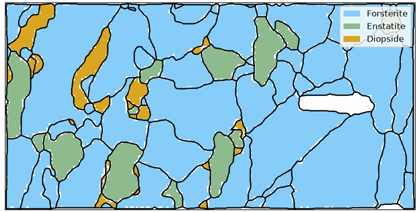
The steps are gone while the larger-scale course of each boundary remains. Smoothing is still a measurement choice rather than recovered sub-pixel truth, and the default filter can shrink grains. How far to smooth and which filter to use are the subject of Grain Boundary Smoothing.

Keeping map and grains together

calcGrains writes one per-pixel property into the map it was given. The grainId property records which grain contains each measurement. Almost every map-to-grain operation in this chapter needs it, and it is there from the first reconstruction on.

grains = calcGrains(ebsd, angle=10 * degree, minPixel=5)

# the measurements inside the largest grain
id = np.argmax(grains.numPixel)
ebsd[grains[id]]

EBSD (y↑→x)
  size: 1624
  Phase  Orientations  Mineral     Color         Symmetry  Crystal reference frame
  1      1624 (100%)   Forsterite  LightSkyBlue  mmm       Forsterite
  properties    : bands, bc, bs, error, grainId, mad
  scan unit     : um
  X × Y         : [5350 → 7750] × [3750 → 7000]
  square lattice: spacing 50

The displayed summary belongs to the measurements in the largest grain, the notIndexed pixels the closing absorbed among them, since they keep their phase. The grain object in ebsd[grains[id]] supplies its stored grain id. That id need not equal its position in a shortened or reordered grain list. Selecting Grains develops this distinction.

The map contains the same measurement positions, but it is not an untouched copy of the import. Removal through minPixel rewrites the phase of the affected measurements. Reconstructing grains from this map a second time is therefore not meaningful; keep ebsd.copy() where the original is still needed.

Grain reconstruction in heavily deformed microstructures

Everything above rests on one assumption: that a misorientation between two neighbouring pixels means the same thing everywhere on the map. A single threshold should then separate “inside a grain” from “across a grain boundary”. In a heavily deformed material that assumption fails from both sides. Inside a grain the lattice is bent. Small neighbour-to-neighbour changes can accumulate to tens of degrees across it. Between two grains, the misorientation may be below any threshold one would call high angle.

We use an austenitic steel deformed in situ. It was indexed by spherical pattern matching rather than by the Hough transform. Its orientation noise is about 0.1 degree. This is roughly one order of magnitude below that of a typical Hough-indexed map, so the deformation substructure is resolved.

plottingConvention.default('y↓→x')
ebsd = mtexdata('EMSphinx')

# the deformed austenite
ebsd = ebsd['Iron fcc']

plot(ebsd, ebsd.orientations, ipfDirection=zvector)

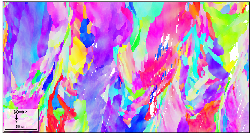
The colour gradients within the elongated grains show the bent lattice. We zoom into a smaller region to see what a threshold makes of it.

region = [40, 30, 80, 60]
ebsd = ebsd[ebsd.inpolygon(region)]

plot(ebsd, ebsd.orientations, ipfDirection=zvector)

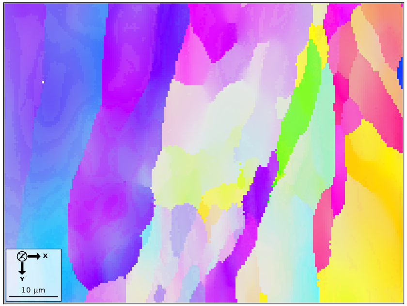
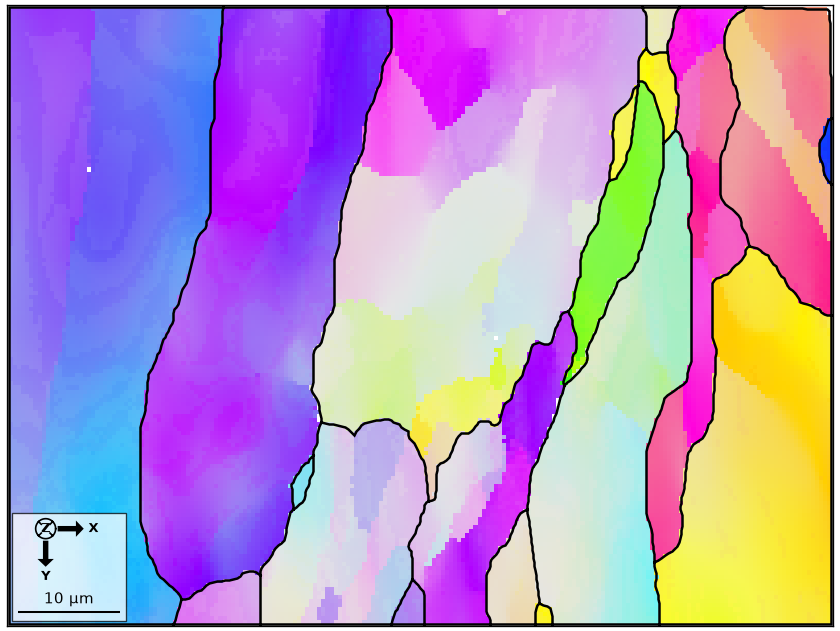
At the usual 10 degree threshold, the reconstruction misses every boundary below that angle. The figure shows several such low-angle boundaries with no black line on them.

grains = smoothBoundary(calcGrains(ebsd, angle=10 * degree, minPixel=10), 5)

plot(ebsd, ebsd.orientations, ipfDirection=zvector)
hold(True)
plot(grains.boundary, lineWidth=1.5)
hold(False)

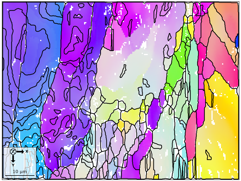
Lowering the threshold does not solve the problem. Before it reaches all the boundary angles of interest, it cuts through the bent lattice inside grains. The dense black lines in the next figure follow contours of the smooth orientation field rather than physical grain boundaries.

grains = smoothBoundary(calcGrains(ebsd, angle=0.5 * degree, minPixel=10), 5)

plot(ebsd, ebsd.orientations, ipfDirection=zvector)
hold(True)
plot(grains.boundary, lineWidth=1.5)
hold(False)

Fast multiscale clustering

The way out is to stop asking about pixel pairs in isolation. Fast multiscale clustering, gbcFMC, builds a hierarchy of progressively coarser pixel aggregates. It fits the lattice gradient within each aggregate. It then compares the residual misorientation between aggregates with their internal orientation spread. A 1 degree step between two uniform aggregates can therefore be a boundary. A comparable step explained by bending within one grain is not. FMC has no threshold angle.

The option fmc selects this criterion. Its value is cmaha. This controls how sharply an unexpected residual misorientation suppresses the coupling between two aggregates. Larger values return more grains.

grains = smoothBoundary(calcGrains(ebsd.copy(), fmc=0.5, minPixel=10), 5)

plot(ebsd, ebsd.orientations, ipfDirection=zvector)
hold(True)
plot(grains.boundary, lineWidth=1.5)
hold(False)

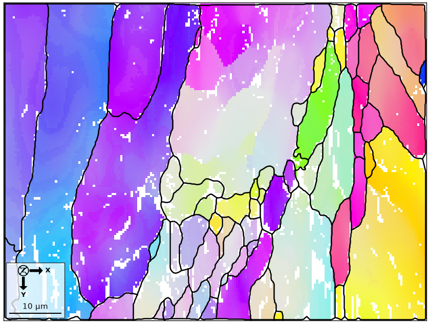
The low-angle boundaries missed by the 10 degree threshold now appear, without the dense spurious contours produced by the 0.5 degree threshold.

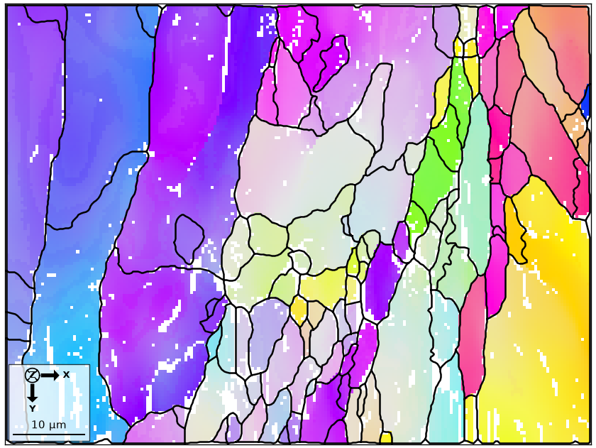
Raising cmaha resolves more of the substructure within those grains, including the dislocation cells that carry the deformation.

grains = smoothBoundary(calcGrains(ebsd.copy(), fmc=1.5, minPixel=10), 5)

plot(ebsd, ebsd.orientations, ipfDirection=zvector)
hold(True)
plot(grains.boundary, lineWidth=1.5)
hold(False)

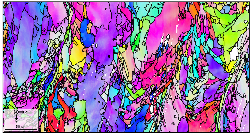
Finally, we apply the same reconstruction to the full map. Unlike a local threshold criterion, FMC clusters the entire map at once rather than one pixel pair at a time, which is why this takes a few seconds. The verbose flag prints how far the hierarchy coarsened and the scales from which the final grains were read.

ebsd = mtexdata('EMSphinx')['Iron fcc']

grains = smoothBoundary(calcGrains(ebsd, fmc=1.5, minPixel=10, verbose=True), 5)

plot(ebsd, ebsd.orientations, ipfDirection=zvector)
hold(True)
plot(grains.boundary)
hold(False)

 fast multiscale clustering of Iron fcc
   478052 pixels, noise 0.108 degree
   cmaha 1.5, cmaha0 0.05, quatmax 5, alpha 0.2, gammaW 10, minPixel 10

 scale   aggregates   gradients   pixels read
 ---------------------------------------------
     1       478052           -             -
     2       189100           0           979
     3        82866         111          2213
     4        36302       11719          5678
     5        16044       12238         11190
     6         7562        6739         24319
     7         4069        3574         42784
     8         2654        2208         68926
     9         2148        1715         72031
    10         1972        1540         89716
    11         1919        1488         85767
    12         1909        1478         34946
    13         1907        1476         36056
    14         1907        1476             0

 3447 pixels read off at no scale

 6553 regions -> 1903 grains, 7017 pixels absorbed into a neighbour, 5 left unassigned

More ways to reconstruct grains

The threshold angle and fast multiscale clustering are two of several criteria by which calcGrains can separate neighbouring pixels. MTEX represents them as interchangeable grainBoundaryCriterion objects. Advanced Grain Reconstruction explains phase-dependent and soft thresholds. It also covers segmentation by another property and custom criteria. Markovian Clustering turns criterion weights into grains in a second way, by clustering the map instead of taking connected components.

Continue with Plotting Grains, then Selecting Grains. The latter uses the grainId relationship established above. The resulting boundary network is the subject of Grain Boundaries.

References

• F. Bachmann, R. Hielscher and H. Schaeben, “Grain detection from 2d and 3d EBSD data - Specification of the MTEX algorithm”, Ultramicroscopy 111 (2011), 1720-1733, doi:10.1016/j.ultramic.2011.08.002. This paper derives the Voronoi-cell reconstruction used by calcGrains.

• C. McMahon et al., “Boundary identification in EBSD data with a generalization of fast multiscale clustering”, Ultramicroscopy 133 (2013), 16-25, doi:10.1016/j.ultramic.2013.04.009.

• R. Hielscher, F. Bartel and T. B. Britton, “Gazing at crystal balls: Electron backscatter diffraction pattern analysis and cross correlation on the sphere”, Ultramicroscopy 207 (2019), 112836, doi:10.1016/j.ultramic.2019.112836. For a direct precision comparison with Hough indexing, see G. Sparks et al., Ultramicroscopy 222 (2021), 113187, doi:10.1016/j.ultramic.2020.113187.

• ISO 13067:2020 describes EBSD measurement of average grain size. It warns that highly deformed specimens require careful interpretation. ASTM E2627-13(2019) applies to fully recrystallised polycrystalline materials. Both make reconstruction choices part of the reported measurement method.

Technical details

calcGrains returns the grains alone and writes grainId into the map it was given, where MATLAB returns a modified copy of the map as its second output; the phases that minPixel marks notIndexed are rewritten in that map too, so a sweep over minPixel on one map passes ebsd.copy(). The alpha closing keeps the phase of every pixel it absorbs, so the sweep over alpha runs on the map itself.

Fast multiscale clustering picks its seeds in order of coupling and aggregate size, and the order of the pixels decides between equal values. MATLAB stores this map with y running fastest, the port with x. Taken in MATLAB’s order, the zoom gives MATLAB’s 55 and 107 grains at cmaha 0.5 and 1.5 and the same hierarchy pair for pair; in the port’s own order it gives 56 and 113. The full map gives 1903 grains, 1900 in MATLAB’s order, for MATLAB’s 1894, in about 14 seconds for MATLAB’s 23.

@article{bachmann2010mtex,
  author  = {F. Bachmann and R. Hielscher and H. Schaeben},
  title   = {Texture Analysis with MTEX - Free and Open Source Software Toolbox},
  journal = {Solid State Phenomena},
  volume  = {160},
  pages   = {63-68},
  year    = {2010},
  doi     = {10.4028/www.scientific.net/SSP.160.63},
  url     = {https://doi.org/10.4028/www.scientific.net/SSP.160.63}
}